It’s Friday night. Our description of the Homo naledi femora (thigh bones) from the Lesedi Chamber is hot off the press. This coincides with the publication of another study (with which I wasn’t involved) of the species’ proximal femur, so I guess you could say it’s a pretty hip time for Homo naledi fossils.

An important task in our study was to estimate the diameter of the poorly preserved femur head (part of the hip joint), a variable which is useful for estimating body mass in extinct animals, which in turn is an important life history variable. One thing I’ve recently been griping about with my students is that while many general research methods are well published, the step-by-step processes usually are not. So, here I’ll detail exactly how we estimated femur head diameter (FHD) —it’s pretty simple, but it took a while to figure it out on my own. And now you won’t have to!
We used the simple yet brilliant approach that Ashley Hammond and colleagues (2013) developed for the acetabulum (the hip socket). In brief, if you have a 3D model or mesh of a bone, you can use various software packages to highlight an area and the software will find the best fit of a given shape to that surface. I used Amira/Avizo and Geomagic Design X, which are great but admittedly quite expensive.
1. Identify the preserved bony surface by making a curvature map
You can do this in Geomagic, but I figured it out in Amira first, so here we are. Also, Amira gives you more control over the resulting colormap, which I think makes it easier to identify preserved vs. broken bone surfaces. The module-based workflow of Amira/Avizo takes some getting used to, but this step is quite simple, once you’ve imported the mesh (“UW 102a-001.stl” in the image below).

Amira workflow (left). The red “Curvature” module is applied to the surface mesh (“UW102a-001.stl”), resulting in a new object (“MaxCurvatureInv”), whose surface view is depicted at right.
The surface is now color-coded, with areas of high curvature (i.e., broken bone and exposed trabecular bone) in blue and better-preserved surfaces in red. This allows you to see which portion(s) of the bone to use to define the sphere.

The curvature map reveals three large patches (A-C) of decently-preserved hip joint surface.
2. Highlight the desired surface in Geomagic
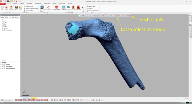
Import the 3D mesh into Geomagic, and use the “Lasso selection mode” to highlight the area (or areas) you wish to fit a sphere to. Make sure that you’ve toggled “Visible only,” so that you don’t accidentally highlight other parts of the bone. You can select a single area, or many areas. In the following example, I’ve highlighted only the large patch (“A” in the previous figure).
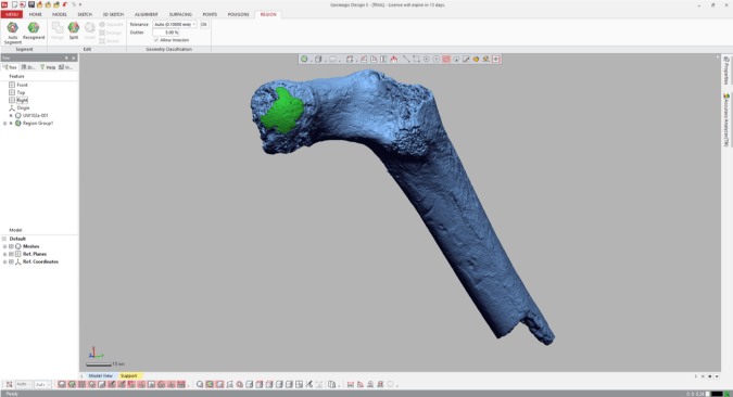
3. Go all Brexit on the highlighted region
That is, declare it as its own distinct region. Navigate to the “Region” tab and click the “Insert” icon. Magically, the highlighted region is now outlined and a shaded in a new color, and listed as “Region group 1” in the window on the left.
4. Measure the region’s radius
Select the “Measure Radius” icon at the bottom of the window, and then when you scroll or hover the mouse over the region, the radius will appear within the patch. The value should be the same throughout the region which is now treated as a spherical surface.

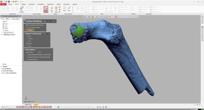
5. Visualize the fitted sphere
If your main goal is to obtain estimates of diameters, you can stop here (don’t forget that the diameter is radius x 2!). But it can be handy to know how the proximal femur would look with the complete head (not that these are perfectly spherical…). To do this, navigate to the “Model” tab and select the “Surface primitive” icon. In the grey menus that appear on the left, select the region and “Sphere” as the shape to be extracted.
Three orthogonal circumferences will appear around the highlighted area, and if they look OK, click the right-pointing arrow at the top of the menus, and there you go!

Wowzers.
I did this a few times on the Homo naledi femur from Lesedi, and got measurements within about 1-2 mm of one another, which is good. What’s more, we used this method on a sample of modern human and fossil hominin femur heads for which the actual diameters were known, to demonstrate the accuracy of the method.

Femur head diameter measured directly (y-axis) vs. sphere-based estimates using the method described here (x-axis). The Homo naledi estimate is indicated by the blue line.
This graph shows that the sphere-based estimates very closely approximate direct measurements, although there is some slight overestimation at larger sizes, i.e. not affecting the H. naledi value. So although the fossil is not perfectly preserved, we are fairly confident in our estimate of its femur head diameter.


