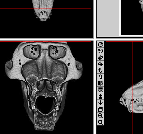
What do capuchin stone tools tell us about human evolution?

October 20, 2016October 20, 2016 / zcofran / 1 Comment

A month ago at ESHE and now online in Nature, Proffitt and colleagues describe stone-on-stone smashing behavior among wild bearded capuchin monkeys (Sapajus libidinosus). The online paper includes a great video documenting the action; here’s a screenshot:

Holding the rock with both hands just above head-level, the monkey prepares to crush its enemies. Which in this case are another rock stuck in a pile of more rocks.

In the fairly rare cases where non-human primates use stones, it’s for smashing nuts or something. But when these capuchins see a stone they don’t just see a smasher, they see a world of possibilities* – why use a rock to break a rock, when you could use it to break a heart? So this group of capuchins is unique in part because they’ve been documented to use stones for many purposes.

Now why on earth a monkey would use one rock to break another rock is anyone’s guess. In human evolution, the purpose was to break off small, sharp flakes that could be used to butcher animals or work plants. Proffitt et al. did observe small flakes being removed when capuchins pounded rocks, but the monkeys showed little interest in this debitage, other than using it to continue smashing stuff. More curiously, the monkeys frequently lick the rock after hammering at it:

Mmm, rocks.

Proffitt et al. venture that maybe these monkeys are doing this to ingest lichens or trace elements like silicon. This hypothesis merits further investigation, but what’s clear is that these monkeys’ lithics differ from the hominin archaeological record wherein the express purpose of breaking rocks is to make flakes.

What’s striking to me (pun intended) is the relative size of the rocks. These monkeys that weigh only 2-3 kg are lifting and smashing stones that weigh about half a kilogram on average. Because these stones are fairly large given the monkeys’ body size, they have to be lifted with two hands and brought down on a surface, a “passive hammer” technique. The earliest-known tools made by hominins, from the 3.3 million year old Lomekwi site in Kenya, are also pretty big. Weighing 3 kg on average but topping at 15 kg, these earliest tools would have required the same knapping technique as is used by these little monkeys (Harmand et al., 2015).

Left: Cover of Nature vol. 521 (7552). Right: Bearded capuchin letting a pebble know who’s boss (link).

Why the big stuff at first? Did the earliest hominin tool-makers lack the dexterity to make tools from the smaller rocks comprising the later Oldowan industry? These creative capuchins could lead to predictions about the hand/arm skeleton of the Lomekwian tool-makers (testable, of course, only with fortuitous fossil discoveries). Capuchins are noted for their manual dexterity (Truppa et al., 2016) and have a similar thumb-index finger ratio to humans and early hominins (Feix et al. 2015), although they differ from humans in the insertion of the opponens muscle and resultant mobility of the thumb (Aversi-Ferreira et al., 2014). Maybe these tech-smart monkeys can tell us more about the earliest human tool-makers’ bodies than their brains.

References

Aversi-Ferreira RA, Souto Maior R, Aziz A, Ziermann JM, Nishijo H, Tomaz C, Tavares MC, & Aversi-Ferreira TA (2014). Anatomical analysis of thumb opponency movement in the capuchin monkey (Sapajus sp). PloS one, 9 (2) PMID: 24498307

Feix T, Kivell TL, Pouydebat E, & Dollar AM (2015). Estimating thumb-index finger precision grip and manipulation potential in extant and fossil primates. Journal of the Royal Society, Interface, 12 (106) PMID: 25878134

Harmand S, Lewis JE, Feibel CS, Lepre CJ, Prat S, Lenoble A, Boës X, Quinn RL, Brenet M, Arroyo A, Taylor N, Clément S, Daver G, Brugal JP, Leakey L, Mortlock RA, Wright JD, Lokorodi S, Kirwa C, Kent DV, & Roche H (2015). 3.3-million-year-old stone tools from Lomekwi 3, West Turkana, Kenya. Nature, 521 (7552), 310-5 PMID: 25993961

Proffitt, T., Luncz, L., Falótico, T., Ottoni, E., de la Torre, I., & Haslam, M. (2016). Wild monkeys flake stone tools Nature DOI: 10.1038/nature20112

Truppa V, Spinozzi G, Laganà T, Piano Mortari E, & Sabbatini G (2016). Versatile grasping ability in power-grip actions by tufted capuchin monkeys (Sapajus spp.). American Journal of Physical Anthropology, 159 (1), 63-72 PMID: 26301957

*well, at least four uses given by Proffitt et al.: mating display, aggression, food-crushing, and digging.

Osteology Everywhere: Why we number our premolars 3-4

November 3, 2015May 30, 2023 / zcofran / Leave a comment

Portishead* came on the radio the other day, making iTunes display the cover of their album, Third. My inner osteologist rejoiced to see it prominently features a tooth!

Third album cover by Porthishead (2008). Image from Wikipedia

Well not a picture, but rather the name, of a tooth. In each quadrant of your mouth (most likely) are two premolars, commonly referred to as “bicuspids.” In the biz, we usually call these pals, “P3” and “P4.”

UW 101-1277 mandible, part of the Homo naledi holotype skull. Modified from the Wits media gallery.

UW 101-1277 mandible, part of the Homo naledi holotype skull. Each capital letter stands for the tooth type (incisor, canine, premolar, and molar). Modified from Wits’ image gallery.

You might be wondering why we call them P3 and P4, when there are only two premolars per quadrant — what happened to P1 and P2? Homology to the rescue!

The ancestral mammalian condition was to have four premolars (and a 3rd incisor) in each side of the jaw. This is a “dental formula” of 3-1-4-3, indicating the numbers of each tooth type from front to back. Over time, different groups of animals have lost some of these teeth. Baleen whales have lost all of them.

P1 and an incisor were lost early in the evolution of Primates. Most Strepsirrhines and Platyrrhine monkeys retain this primitive”2-1-3-3″ dental formula :

Ring tailed lemur (left) and woolly monkey (right) maxillae, showing the primitive primate dental formula including a P2. For scale, gridlines are 10 mm (left) and 20 mm (right). Images from this boss database.

The last common ancestor of catarrhines (living humans, apes and Catarrhine monkeys) lost the P2, and so we have only two premolars left in each side of the jaw. These are homologous with the third and fourth premolars of the earliest mammals. And that’s why we call them P3-4.

*The song was “The Rip.” It’s a very good song with an insanely creepy and trippy video:

Bioanthro lab activity: Primate proportions

September 28, 2015October 26, 2015 / zcofran / Leave a comment

My Intro to Bio Anthro course, focusing on human uniqueness, has moved from the brain to bipedalism. After the abysmally big brain, perhaps the most grotesque aspect of the human species is our wont to walk on two legs. It’s just not natural.

What a terrible biped. Image credit.

Seriously, why would an animal do such a horrid thing?

Most animals need extra help to stay upright on just two limbs. Image credit.

This peripatetic penchant is apparent in our skeletons, most visibly in our long-ass legs. And indeed, species’ limb lengths and proportions generally reflect how they tend to move around. Quadrupeds, animals that walk on four legs, tend to have roughly equally-lengthed arms and legs. Gibbons, notorious ricochetal brachiators, have insanely long arms. So for lab this week, students measured surface scans of different primates’ long bones to see if form really follows function.

Here, students try their hands at measuring long bones on surface scans of primate skeletons, and use their data to calculate indices reflecting the relative lengths of limb segments. These data will be used to test whether limb proportions can be used to distinguish different locomotor types, and to hypothesize how fossil species might have moved about.

Measuring siamang (Symphalangus syndactylus) limb lengths with Meshlab. Data credit.

Since this is my students’ introduction to primate skeletons and analysis software, I only had them measure three specimens: a siamang (above), a squirrel monkey, and a grivet. But of course you can have students look at more if you wish. This activity uses the free Meshlab software and surface scans made from CT scans in the KUPRI database (surface scans are much smaller files than CT scans, making for easier dissemination to swarms of students). If you’re interested in using or modifying this activity in your class, here are the lab handout and datasheet I created for it:

Lab 2-Primate proportions
Lab 2-Primate limb data sheet

Info about, and materials for, other lab activities can be found on my Teaching page.

Online primate anatomy lab exercise

February 5, 2014February 6, 2014 / zcofran / 3 Comments

I work at a very freshly opened University in Kazakhstan, a school so young that we will not graduate our first class for another year. I came here for the exciting prospects of helping establish an anthropology program, but there are lots of challenges, too. One of the biggest I face as an educator is that infrastructure and other physical materials are still in the process of coming together. Simply put: we don’t got no bones! This is especially troublesome when teaching human evolution, an anatomy-oriented class in which students really can benefit from examining physical bones and casts of fossils first-hand.

So until we get our badass laboratory of anthropological sciences, I’ve put together a lab activity using the Kyoto University Primate Research Institute’s online database of CT scans (blogged about before here and here). The purpose of this activity is to show students ‘virtual’ primate skeletons that they can examine, look inside, and even measure. The KUPRI CT viewers allow students to identify structures, rotate and orient the skeletons, and measure using a handy grid function. While I love this resource, I’ll admit that the program can be a bit unwieldy, and so it takes some time to figure out how to use well.

Measure that gibbon radius!

In this exercise, students will measure cranial width, femur head diameter, and maximum length of the humerus, radius, femur, and tibia. Cranium width is then used to estimate cranial capacity (based on chimps, from Neubauer et al., 2012); femur head diameter allows estimation of body mass (using anthropoid regressions from Ruff, 2003); and the limb dimensions are used to calculate various indices. The class as a whole will look at apes and monkeys, for comparison with published values for other species. Then we’ll gather ’round the campfire to talk about our feelings about it. I’m hoping it will get them familiar with the basic anatomy and names of bones, some experience collecting data, and some understanding of variation between different species.

Best of all, each student will write up their ‘analysis’ on the NU Bioanthro Student blog next week. Stay tuned to see their results!

So, I’m attaching the exercise to this post – feel free to use or modify. If you have any other similar exercises, the rest of the internet and I would be happy to hear about them

Download me: Primate CT lab! [updated 06 Feburary, to fix issues with brain and body size estimation equations in previous version]

Look inside bones for free on the interwebs

November 20, 2011August 4, 2013 / zcofran / 2 Comments

I forget how I stumbled upon this badass resource, but Kyoto University’s Primate Research Institute made a “Digital Morphology Museum: an awesome online database of CT scans of sundry primate skeletal parts. Ever wonder what an articulated siamang skeleton looks like? Or whether the flaring bony snout of a mandrill is hollow or filled with bone (below)? If you’re a normal person, probably not. But either way, this website provides easy access to the internal views of all sorts of body parts.

Coronal slice through a male mandrill face. You can see a bone-filled lower jaw, internal views of some teeth, the nasal cavity. The pics above and on the right give an idea of where in the skull we are. Note the fat flanks above the nasal cavity are filled with bone (they hollow out as you move further into the face).

What’s cool is you can view and manipulate 3D views of these things on the website, or you can register with KUPRI to download the raw CT data. Really a great resource.

A few weeks ago, a paper came out wherein researchers used CT scans to compare the the sides of the nasal opening in skulls of Australopithecus species (Villmoare and Kimbel 2011). They found that although the external nose of the South African Australopithecus africanus and A. robustus appear similar in looking like rounded “pillars,” on the inside these pillars differed between the two species. A. africanus‘s (and the earlier, east African A. afarensis‘s) nasal pillar was hollow, while A. robustus‘s was filled with “spongy” bone, like the contemporaneous A. boisei in East Africa. So the early (and “gracile”) australopiths had hollow pillars while the later (and “robust”) ones had a bony pillar, hmm… It’d be neat to try to see how such bone-filled or hollow pillars develop (i.e. are they hollow in babies but then fill with trabecular bone during growth in the “robust” group? Does this difference arise for functional (e.g. chewing) reasons, or could it be a developmental ‘byproduct’ of the tall robust australopithecine face [cf. McCollum 1999]).

It’s a neat study, and they include lots of great CT images of the hominid sample. But another question arises – what is the inside of the bony nose like in modern primates, and how much variation is there within a species? (NB Villmoare and Kimbel found pretty much no variation within each fossil species, save for two curious examples, but which were based on casts). If I had the time (i.e. weren’t dissertation-ating) I’d love to peruse the KUPRI files to see what “pillar” variation is like in, say, chimps (paleoanthropologists’ go-to referent species). Cursorily looking at just one (female chimpanzee, left), it looks like the sides of the nose are empty higher up, but then fill with bone to form the tooth socket surrounding the canine root. I’ll leave it to someone else to see what the rest look like.

But just lookit what other fun stuff you can see! At the top (anatomically toward the back) are the bone-filled mandibular condyles, beneath (anatomically a bit more toward the front) and between them are the pterygoid plates, and beneath them is a big gross maxillary sinus. Man, if only I had the time, I’d make an anatomy scavenger hunt on this site, and it’d be pretty epic.

Those papers I mentioned
McCollum, M. (1999). The Robust Australopithecine Face: A Morphogenetic Perspective Science, 284 (5412), 301-305 DOI: 10.1126/science.284.5412.301

Villmoare, B., & Kimbel, W. (2011). CT-based study of internal structure of the anterior pillar in extinct hominins and its implications for the phylogeny of robust Australopithecus Proceedings of the National Academy of Sciences, 108 (39), 16200-16205 DOI: 10.1073/pnas.1105844108

Stimulating the drunk on the platform

March 2, 2011August 4, 2013 / zcofran / Leave a comment

Gotcha! I mean “simulating” in the title, not “stimulating.” This one’s about programming.

I’m interested, for various reasons, in how evolution might bring about change over time. Recall from my Evolution Overview that evolutionary changes could occur by drift or natural selection. Drift means random change, because a given polymorphism has no effect on fitness. Natural selection, on the other hand, is what my advisor likes to call the 900-lb gorilla: it does whatever the eff it wants. Selection can take existing variation in a population and mold it into all kinds of oddities. Within Primates, natural selection has fashioned inquisitive apes that walk on two legs and go to the moon, and sexual selection has festooned male mandrills in variegated visage (right). Selection can be gentle and allow gradual change (what I like to call sensual selection), or it could be strong and cause rapid change.

Selection can seem random for various reasons (e.g. why is it acting as intensely as it does when it does?), so it is hard to tell whether a given evolutionary scenario can be explained by selection for a given behavior, or if it reflects totally random change (drift).

Monte Carlo statistical methods allow one to simulate a given scenario, to test competing hypotheses. A simple null hypothesis that can be simulated is drift – change is completely random in direction, and if I reject this hypothesis I could argue that an alternative explanation (selection) is appropriate

The random walk is the oft-used analogy for this null hypothesis of random change. Now, if I’d ever been so imperfect as to have succumbed to the siren-song of spirits, maybe I’d corroborate the analogy. But using the extent of your limited but unadulterated imagination, pretend there is a drunk kid who happened to go to Loyola Chicago (like myself), and who walks onto the L platform (like I often did; left, looking north from the Lawrence Red Line stop). As booze takes the reins, he stumbles randomly between the edges of the train platform. This random walk down the train platform could result in the drunkard making it safely to the end, or he could fall off either side to a gruesome doom awaiting on the tracks below.

Thinking about limb proportions, and how to program this hypothesis/scenario, I stumbled upon the useful cumsum() function for the R statistical program. This function allows me to indicate how much change to occur for how many steps (i.e. generations), thus effectively simulating the random walk. For example (right), say I want to ask if the tibia (shin bone) gets long relative to the femur (thigh bone) in human evolution, because of drift vs. natural selection. I start with a given proportion of [tibia/femur] and simulate change in a random direction in tibia and femur length, over a quarter million years (or 18,000 15-year generations).

The figure is a bird’s eye view of a random walk: at each generation the drunken tibia/femur ratio steps forward (to the right in the picture) and randomly right or left (toward the top or bottom of the picture). This took literally 2 seconds to program and graph. The dashed black line represents the relative tibia/femur relationship at the beginning of the evolutionary sequence, and the red line is the ratio 250,000 years (18,000 generations) later. Note that in this particular random scenario, not only is the final tibia/femur ratio exactly that observed, but that over the time span this ratio was reached about 20 different times. Do this randomization 500 or more times to see how often random change will result in the observed difference between time periods. Assuming the simulations realistically model reality, the observed change in limb proportions could easily be explained by drift (i.e. climate or efficiency adaptations did not have so strong a selective advantage as to be detected by this test). That is, the change in proportions could have been effected by random change or by weak directional selection.

I’m currently looking for any ways to make the model more realistic, for example:

how much evolution (e.g. change) could occur per generation. Currently, each generation changes by plus or minus a given maximum. I would like to be able to simulate any amount of change between zero and an a priori maximum.
it’s easier to let the tibia and femur change randomly with respect to one another. However, this is unrealistic because the thigh and leg are serially homologous, their variation is not independent of one another. I would like to model each element’s change per generation to reflect this covariance.

Anyway, I’ve only begun looking into the topic of how to analyze evolutionary change, but it looks like testing evolutionary hypotheses might not be impossible?

This just in: Primates have differently shaped skulls

February 24, 2010 / zcofran / 1 Comment

Sorry for the lag in posting. This semester’s been quite busy and hectic, as I’m trying really now to figure out what I’m doing here in graduate school. But I just had to stop what I’m doing to let everyone know about this ground-breaking discovery.

A study just published in the American Journal of Physical Anthropology has used the powerful shape-analysis technique of geometric morphometrics to discover that primate crania are quite diverse! Sampling one male and one female from a wide variety of primate genera, the researchers determined the shape-differences among these major groups using 3D landmark coordinates and principle components analysis. Wouldn’t you know, that their analysis showed a clear distinction between strepsirhines (lemurs and lorises, the most primitive of all primates) and anthropoids (monkeys and apes, which includes humans). Oh, and humans are markedly different from our ape brethren. So now all those speciesists out there can’t claim that, “all primates look alike.”

Why is this paper interesting? Um…

Reference

Fleagle J, Gilbert C, and Baden A. Primate Cranial Diversity. American Journal of Physical Anthropology, in press.

Lawn Chair Anthropology

Biological anthropology, paleontology, evolution, and development, by Dr. Zachary Cofran

primates