#AAPA2017 – Modularity & evolution of the human canine

I’m recently returned from this year’s AAPA Conference, hosted by Tulane University in New Orleans. What a trip!

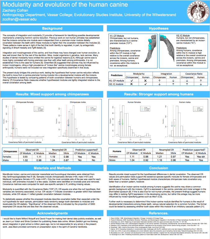
Usually my presentations involve fossils and/or growth, but this year I wanted to try a different way of looking at the evolution & development – integration & modularity. In short, biological structures that share a common developmental background and/or function may comprise ‘modules’ that are highly ‘integrated’ with one another, but relatively less integrated with other structures or modules.

I hypothesized that canine reduction in hominins is a result of a shift in modularity of the dentition, such that the canine became more highly integrated with the incisors than with the premolars. I’d thought of this 5 years ago when creating the first rendition of my human evo-devo course (offering again next fall!), but never got to look into it. Interestingly, the results generally supported my predictions, except for one pesky sample…

Screen Shot 2017-04-23 at 8.36.05 AM

As my primatologist friends will tell you, male chimps are the worst.

Here’s a pdf version of the poster. It was fun to dabble with a new methodology, to see my far-flung friends, and to visit a fun historic place for the AAPA conference. Definitely looking forward to next year in Austin!

Materials from the R workshop at #AAPA2016

For last week’s AAPA conference, my friend and colleague David Pappano organized a workshop teaching about the many uses of the R programming language for biological anthropology (I’m listed as co-organizer, but really David did everything). After introducing the basics, we broke into small groups focusing on specific aspects of using R. I devised some lessons for basic statistics, writing functions, and resampling. Since each of the lessons could have easily taken up an hour and most people didn’t get to go through the activities fully, I’m posting up the R codes here for people to mess around with.

The basic stats lesson utilized Francis Galton’s height data for hundreds of families, courtesy of Dr. Ryan Raaum. To load in these data you just need to type into R: galton = read.csv(url(“http://bit.ly/galtondata“)). The code simply shows how to do basic statistics that are built into R, such as  t-test and linear regression.

Example of some summary stats for the Galton height data.

Some summary stats for the Galton  data. The code is in blue and the output in black.

Here is the Basic Stats code, download and paste it into an R file, then buckle up!

The lesson on functions and resampling was based on limb length data for apes, fossil hominins and modern humans (from Dr. Herman Pontzer). The csv file with the data can be downloaded from David’s website. R has lots of great built-in functions (see basic stats, above), and even if you’re looking to do something more than the basics, chances are you can find what you’re looking for in one of the myriad packages that researchers have developed and published over the years. But sometimes it’s necessary to write a function on your own, and with fossil samples you may find yourself needing to do resampling with a specific function or test statistic.

For example, you can ask whether a small sample of “anatomically modern” fossil humans (n=12) truly differs in femur length from a small sample of Neandertals (n=9). Traditional statistics require certain assumptions about the size and distribution of the data, which fossils fail to meet. Another way to ask the question is, “If the two groups come from the same distribution (e.g. population), would random samples of sizes n=12 and n=9 have so great an average difference as we see between the fossil samples?” A permutation test, shuffling the group membership of the fossils and then calculating the difference between the new “group” means, allows you to quickly and easily ask this question:

R code for a simple permutation test.

R code for a simple permutation test. The built-in function “sample()” is your best friend.

Although simply viewing the data suggests the two groups are different (boxplot on the left, below), the permutation test confirms that there is a very low probability of sampling so great a difference as is seen between the two fossil samples.

Left: Femur lengths of anatomically modern humans (AMH) and Neandertals. Right: distribution of resampled group differences. Dashed lines bracket 95% of the resampled distribution, and the red line is the observed difference between AMH and Neandertal femur lengths. Only about 1% of the resampled differences are as great as the observed fossil difference.

Left: Femur lengths of anatomically modern humans (AMH) and Neandertals. Right: distribution of resampled group differences. Dashed lines bracket 95% of the resampled distribution, and the red line is the observed difference between AMH and Neandertal femur lengths. Only about 1% of the resampled differences are as great as the observed fossil difference.

Here’s the code for the functions & resampling lesson. There are a bunch of examples of different resampling tests, way more than we possibly could’ve done in the brief time for the workshop. It’s posted here so you can wade through it yourself, it should keep you busy for a while if you’re new to R. Good luck!
R workshop at #AAPA2016

The 85th annual meeting of the American Association of Physical Anthropologists, in Hottlanta this year, is only a few short weeks away. The preliminary program is up, and there’s really a lot to look forward to at this year’s conference. There’s a session dedicated to Homo naledi on Saturday morning (16 April), and I’ll be presenting on dental development in Homo naledi at the very end of the last session of the day. Leading up to the conference, I’ll be tweeting teasers as I put together my talk.

My colleague David Pappano and I are also organizing a workshop on using R in biological anthropology, which will take place on Friday 15 April from 9:30-11:30 am. The goal of the workshop isn’t to make you an expert in R by the end of the two short hours, but rather to introduce you to the basic functions and potential uses of the powerful, free statistical software. So if you’Re Ready to leaRn some R basics, come to Room A601 on FRiday moRning – it’s fRee and no RegistRation is RequiRed.

Hopefully we’ll see you in Atlanta in a few weeks!

#AAPA2015

Tomorrow I’m heading to St. Louis, MO for the annual meeting of the American Association of Physical Anthropologists. I’ll be giving a talk on Saturday presenting results of a comparison of brain size growth between captive and wild chimpanzees. Some recent work has highlighted differences between captive and wild animals in terms of bodily growth and maturation, but so far as I know brain development has not been part of this. Here’s a teaser plot, showing how the captive (blue) and wild (green) datasets deviate from a piecewise linear regression of brain size against age (for the combined wild+captive sample):

Rplot copyThe dashed black line is zero, or no deviation from the model. This plot shows that each dataset deviates little from the model at younger ages (when the brain is growing rapidly), but at older ages the captive animals have larger brains, and the wild animals have smaller brains, than predicted by the model. What’s the meaning of this? Find out Saturday afternoon at 3 pm…

2015 AAPA conference: More brain growth

The American Association of Physical Anthropologists is holding its annual meeting next year in St. Louis, in my home state of Missouri (I’m from Kansas City, which is by far the best city in the state, if not the entirety of the Midwest). I’ll be giving a talk comparing brain size growth in captive and wild chimpanzees, on Saturday 28 March in the Primate Life History session. Here’s a sneak peak:

Velocity curve for brain size from birth to 5 years in wild (green) and caprive (blue) chimpanzees. For the captive models, the dashed line is fit to the raw brain masses, and the solid line is fit to the estimated endocranial volumes.

Velocity curves for brain size growth from birth to 5 years in wild (green) and captive (blue) chimpanzees. The wild data are endocranial volumes, but the captive specimens are represented by brain masses. So the captive data are modeled for both the original masses (dashed) and estimated volumes (solid). Wild data are from Neubauer et al. 2011, captive data from Herndon et al., 1999.

Abstract: This study compares postnatal brain size change in two important chimpanzee samples: brain masses of captive apes at the Yerkes National Primate Research Center, and endocranial volumes (ECVs) of wild-collected individuals from the Taï Forest. Importantly, age at death is known for every individual, so these cross-sectional samples allow inferences of patterns and rates of brain growth in these populations. Previous studies have revealed differences in growth and health between wild and captive animals, but such habitat effects have yet to be investigated for brain growth. It has also been hypothesized that brain mass and endocranial volume follow different growth curves. To address these issues, I compare the Yerkes brain mass data (n=70) with the Taï ECVs (n=30), modeling both size and velocity change over time with polynomial regression. Yerkes masses overlap with Taï volumes at all ages, though values for the former tend to be slightly elevated over the latter. Velocity curves indicate that growth decelerates more rapidly for mass than ECV. Both velocity curves come to encompass zero between three and four years of age, with Yerkes mass slightly preceding Taï ECV. Thus, Yerkes brain masses and Taï ECVs show a very similar pattern of size change, but there are minor differences indicating at least a small effect of differences in habitat, unit of measurement, or a combination of both. The overall similarity between datasets, however, points to the canalization of brain growth in Pan troglodytes.

My ESHE poster is Gona blow your mind

I’m in Italy for the annual meeting of the European Society for the Study of Human Evolution. It’s been a great conference, seeing interesting talks (check out #eshe2014 on Twitter), meeting old friends and meeting new ones, and enjoying excellent food and espresso. Here’s the poster I presented yesterday (download pdf):Screen Shot 2014-09-20 at 9.33.38 AM

It’s a follow-up to posts here and here. The long and short of it is, there was a substantial amount of body size variation (i.e., between males and females) in Homo erectus, on par with levels seen in modern day gorillas. This is interesting because H. erectus brain size (and brain size growth) would have required massive amounts of energy, so some have hypothesized a cooperative breeding strategy; sexually dimorphic species generally do not engage in such cooperative behavior. So I suggest that body size variation in H. erectus is an ecological strategy, with small female body size reducing the metabolic burden on mothers.

#AAPA2014

I’ve jumped across some continents, to Calgary for the 83rd annual meeting of the American Association of Physical Anthropologists. It’s a frenetic few days to catch up with close friends and colleagues, and to discuss upcoming projects. Also hopefully there will be poutine. You can follow the conference goings-on on Twitter with the hashtag #AAPA2014.

I’ll be presenting some work I began last summer (first blogged here), as part of a symposium in honor of Alan Mann. Mann was one of the first researchers to point out the similarities in dental development between humans and australopithecines, and his book Some Paleodemographic Aspects of the South African Australopithecines (1975) was an important resource in my dissertation research. In my current project, I try to identify traits in the lower jaw that follow a similar pattern of size growth as the rest of the body, to reconstruct growth in extinct species that are represented mostly by jaw fossils.

If you’re interested in what I’ve found, come and find me at my poster Saturday afternoon. If you can’t make it, here’s the poster I’ll be presenting:

AAPA 2014 Poster

AAPA 2014 Poster


Is Boas Dead?! Anthropology graduate conference

The University of Michigan’s Anthropology graduate association (MAGA) is hosting a FREE anthropology conference here in Ann Arbor this coming Saturday, 27 March. The event is titled, “Is Boas Dead?! Four-field anthropology in the 21st Century,” (click the title for the link) and will feature a day of anthropology talks in all four fields (well, archaeology didn’t really represent, unfortunately).

Four members of this blog will be presenting at this conference. I myself will be presenting at the end of the day, in a talk fairly mundanely titled, “Population-specific variation in studies of integration.” Basically, variation is a natural part of human populations. However, some populations are more variable than others. The question I ask is whether variation unique to populations poses a problem for studies of integration, which are based on correlations between traits, usually in large, pooled samples containing individuals from all over dodge. The answer to the question is, ‘yes and no.’
So if you can make it out, come see what the Michigan anthropology graduate students are up to! It’s free, and better yet, educational! Or maybe the free part is more exciting.