Brain size & scaling – virtual lab activity

Each year in my intro bio-anthro class, we start the course by asking how our brains contribute to making us humans such quirky animals. Our first lab assignment in the class uses 3D models of brain endocasts, to ask whether modern human and fossil hominin brains are merely primate brains scaled up to a larger size. In the Before Times, students downloaded 3D meshes that I had made, and study and measure them with the open-source software Meshlab. But since the pandemic has forced everyone onto their own personal computers, I made the activity all online, to minimize issues arising from unequal access to computing resources. And since it’s all online, I may as well make it available to everyone in case it’s useful for other people’s teaching.

The lab involves taking measurements on 3D models on Sketchfab using their handy measurement tool, and entering the data into a Google Sheets table, which then automatically creates graphs, examines the scaling relationship between brain size (endocranial volume, ECV) and endocast measurements, and makes predictions about humans and fossil hominins based off the primate scaling relationship. Here’s the quick walk-through:

Go to the “Data sources” tab in the Google Sheet, follow the link to the Sketchfab Measurement Tool, and copy the link to the endocast you want to study (3D models can only be accessed with the specific links).

Following the endocast Sketchfab link (column D) will bring you to a page with the 3D endocast, as well as some information about how the endocast was created and includes its overall brain size (ECV in cubic cm). Pasting the link when prompted in the Measurement Tool page will allow you to load, view, and take linear measurements on the endocast.

Hylobates lar endocast, measuring cerebral hemisphere length between the green and red dots.

Sketchfab makes it quite easy to take simple linear measurements, by simply clicking where you want to place the start and end points. The 3D models of the endocasts are all properly scaled, and so all measurements that appear in the window are in millimeters.

The assignment specifies three simple measurements for students to take on each endocast (length, width, and height). In addition, students get to propose a measurement for the size of the prefrontal cortex, since our accompanying reading (Schoenemann, 2006) explains that it is debated whether the human prefrontal is disproportionately enlarged. All measurements are then entered into the Google Sheet — I wanted students to manually enter the ECV for each endocast, to help them appreciate the overall brain size differences in this virtual dataset (size and scale are often lost when you have to look at everything on the same-sized 2D screen).

Feel free to use or adapt this assignment for your own classes. The assignment instructions can be found here, and the data recording sheet (with links to endocast 3D models) can be found here — these are Google documents that are visible, but you can save and edit them by either downloading them or making a copy to open in Docs or Sheets.

Ah, teaching in the pandemic 🙃

Latest from the lab: Brain size at Krapina

In the latest paper out of the lab (here), my students and I reconstructed the brain endocasts of the Krapina Neandertals. The Krapina rock shelter in Croatia is a remarkable site. Dating to around 130,000 years ago (if not older), the Krapina fossils are early members of the Neandertal lineage. In addition, the fossils represent dozens of Neandertals, from infants to adults. Part of what drew me to the site were the juvenile skulls, since they can tell us about growth and development in these early humans. But, the fossils are quite fragmentary, and needed to be reconstructed to estimate important characteristics like brain size.

Figure 1 from our paper, showing the five Krapina crania (A & B are the same individual) with the endocranial surface highlighted.

Vassar College has a great program called URSI, where students team up with faculty to get hand on experience conducting research over the summer. So, two summers ago my students and I worked on virtually putting these Humpties Dumpty back together again. Using 3D surface scans of the original fossils and CT scans of modern humans, we used virtual methods to digitally reconstruct the endocasts, which are a good proxy for brain size and shape. Here’s the basic workflow:

Figure 2 from the paper, depicting the workflow for virtually reconstructing fossil endocasts, represented by the famous Krapina 3 or “C” cranium.

The human endocasts were produced from recent humans from the Terry Anatomical Collection, generously made available here by Dr. Lynn Copes. We have posted the 3D landmark data for the humans, the preserved landmarks from the Neandertals, and a big list of estimated brain sizes for Neandertals, in the open access repository Zenodo (here). So, hopefully anyone can repeat our results, or use these data in their own research.

With virtual methods, we could generate multiple reconstructions of each Neandertal fairly easily, giving an idea of how certain or uncertain our brain size estimates were. In the end, we showed that i) the Krapina juveniles, who were probably around 6-7 years old, had brain sizes within the adult range (it’s same with modern humans); ii) average brain size at Krapina was a little lower than previously estimated; and iii) although later Neandertals from other sites had larger brains on average, the difference is not necessarily greater than could be expected by chance.

I’ve participated in Vassar’s URSI program for the past few years and it has been a lot of fun. Last (virtual) summer, my students and I compared hip growth in humans and Australopithecus africanus, and this coming summer we will examine the brains of the greatest animals of all time — gibbons!

This is how we do it

It’s Friday night. Our description of the Homo naledi femora (thigh bones) from the Lesedi Chamber is hot off the press. This coincides with the publication of another study (with which I wasn’t involved) of the species’ proximal femur, so I guess you could say it’s a pretty hip time for Homo naledi fossils.

screenshot_116

An important task in our study was to estimate the diameter of the poorly preserved femur head (part of the hip joint), a variable which is useful for estimating body mass in extinct animals, which in turn is an important life history variable. One thing I’ve recently been griping about with my students is that while many general research methods are well published, the step-by-step processes usually are not. So, here I’ll detail exactly how we estimated femur head diameter (FHD) —it’s pretty simple, but it took a while to figure it out on my own. And now you won’t have to!

We used the simple yet brilliant approach that Ashley Hammond and colleagues (2013) developed for the acetabulum (the hip socket). In brief, if you have a 3D model or mesh of a bone, you can use various software packages to highlight an area and the software will find the best fit of a given shape to that surface. I used Amira/Avizo and Geomagic Design X, which are great but admittedly quite expensive.

1. Identify the preserved bony surface by making a curvature map
You can do this in Geomagic, but I figured it out in Amira first, so here we are. Also,  Amira gives you more control over the resulting colormap, which I think makes it easier to identify preserved vs. broken bone surfaces. The module-based workflow of Amira/Avizo takes some getting used to, but this step is quite simple, once you’ve imported the mesh (“UW 102a-001.stl” in the image below).

step 1

Amira workflow (left). The red “Curvature” module is applied to the surface mesh (“UW102a-001.stl”), resulting in a new object (“MaxCurvatureInv”), whose surface view is depicted at right.

The surface is now color-coded, with areas of high curvature (i.e., broken bone and exposed trabecular bone) in blue and better-preserved surfaces in red. This allows you to see which portion(s) of the bone to use to define the sphere.

Screen Shot 2019-06-26 at 10.55.28 AM

The curvature map reveals three large patches (A-C) of decently-preserved hip joint surface.

2. Highlight the desired surface in Geomagic
Import the 3D mesh into Geomagic, and use the “Lasso selection mode” to highlight the area (or areas) you wish to fit a sphere to. Make sure that you’ve toggled “Visible only,” so that you don’t accidentally highlight other parts of the bone. You can select a single area, or many areas. In the following example, I’ve highlighted only the large patch (“A” in the previous figure).

Screen Shot 2019-06-26 at 11.25.59 AM

3. Go all Brexit on the highlighted region
That is, declare it as its own distinct region. Navigate to the “Region” tab and click the “Insert” icon. Magically, the highlighted region is now outlined and a shaded in a new color, and listed as “Region group 1” in the window on the left.

Picture1

4. Measure the region’s radius
Select the “Measure Radius” icon at the bottom of the window, and then when you scroll or hover the mouse over the region, the radius will appear within the patch. The value should be the same throughout the region which is now treated as a spherical surface.

Screen Shot 2019-06-26 at 12.19.36 PM

5. Visualize the fitted sphere
If your main goal is to obtain estimates of diameters, you can stop here (don’t forget that the diameter is radius x 2!). But it can be handy to know how the proximal femur would look with the complete head (not that these are perfectly spherical…). To do this, navigate to the “Model” tab and select the “Surface primitive” icon. In the grey menus that appear on the left, select the region and “Sphere” as the shape to be extracted.

Picture1

Three orthogonal circumferences will appear around the highlighted area, and if they look OK, click the right-pointing arrow at the top of the menus, and there you go!

Picture1

Wowzers.

I did this a few times on the Homo naledi femur from Lesedi, and got measurements within about 1-2 mm of one another, which is good. What’s more, we used this method on a sample of modern human and fossil hominin femur heads for which the actual diameters were known, to demonstrate the accuracy of the method.

Lesedi sphere vs FHD_No Krapina copy

Femur head diameter measured directly (y-axis) vs. sphere-based estimates using the method described here (x-axis). The Homo naledi estimate is indicated by the blue line.

This graph shows that the sphere-based estimates very closely approximate direct measurements, although there is some slight overestimation at larger sizes, i.e. not affecting the H. naledi value. So although the fossil is not perfectly preserved, we are fairly confident in our estimate of its femur head diameter.

A change of scenery

It’s been quiet here as I’ve been moving the Lawnchair all over the place since the summer and haven’t had time to write. Bittersweetly no longer in Kazakhstan, I’ve just joined the Anthropology Department at Vassar College in New York. Here’s a quick, summery summary of one of the last things I did as an immigrant in Central Asia.

Site search: No end in sight

Screen Shot 2016-09-04 at 1.42.03 PM

The yellow pin marks the location of our survey. This is very close to the Polygon, a nuclear test site used during Soviet times.

In early June some colleagues and I ventured to East Kazakhstan in search of caves that earlier humans might have called home. Our initial plan was to visit the Altai Mountains, but permits fell through at the last minute. Fortunately, Bronze Age archaeologists from Eurasian National University and University of Semipalatinsk told us of some caves near where they were working in the Shyngystau region, and let us set up camp with them.

DSC06851

Lightning strikes behind the karstic, cave-pocked uplift by our campsite.

Abutting Bronze Age burial mounds and just a small hike to a large recent cemetery, the campsite was flanked by thousands of years of burial practices. Would the nearby caves push this boundary into the Stone Age?

DSC06863.JPG

Looking south from the previously pictured caves. Trees mark the course of a braided stream, and in the distance you can barely make out the mausoleum-filled cemetery. Camp is just off-camera to the right.

We found and explored a number of shallow caves in the area, but unfortunately none of these were productive Paleolithic sites. This rocky uplift (below), for instance, was adjacent to a meandering stream that probably gets pretty deep during flood season. The water had carved out one small cave (bottom right), and there was a larger, south-facing cave just above ground level.

DSC06903.JPG

The larger cave funneled into an enticingly narrow crawlspace. On the principle of “if you don’t look, you’ll never know,” and inspired by the geological situation of Homo naledi, we figured it was worth at least looking.

WRONG! It ended when I was only a little over a body length in. But again, if you don’t look, you’ll never know. What you will come to know, however, is how many and what size of spiders are in cave; the result is always upsetting.

Spiders 2.JPG

While the trip didn’t go exactly as planned, it was still highly informative to see more of the geology of East Kazakhstan. Fortunately, we have received funding from the Growth Development and Research Institute of Nazarbayev University, to begin survey of the Bukhtarma River Valley as we’d initially intended. Hopefully next summer we’ll see more caves, exciting finds, and fewer spiders.

Osteology Everywhere: Ardipithecus in Almaty?

A few weeks ago I was traipsing across Almaty, Kazakhstan’s former capital, when a stain in the road caught my eye:

2016-05-06 20.11.56

Roadside osteology. The intersection of the trunk and legs at the intersection of Abay & Seifullin?

It’s obviously iliac but it’s not just any old ilium. I think I discovered the underreported antimere of the Ardipithecus ramidus pelvis (ARA-VP 6/500; Lovejoy et al., 2009). What it’s doing in Almaty, and in the middle of a busy street, I have no idea. I’ve long thought the absence of hominin fossils in Kazakhstan was suspicious. But not this suspicious.

Roadside paleontology. The Almaty Ardi innominate (left), compared with the actual ARA-VP-1/500 innominate (center) and its reconstruction (right). Adapted from Lovejoy et al. 2009.

Roadside paleontology. The Almaty intersection innominate (left), compared with the actual ARA-VP-1/500 innominate (center) and its reconstruction (right). Adapted from Lovejoy et al. 2009.

The Ardi innominate pictured (center, above) is from the left side, and the Almaty intersection innominate is a perfect counterpart from the right. Yes, I know they found a right ilium at Aramis to go with the better preserved left half. But to that I reply:

ModernFamily-Shame-GIF

Let’s compare the “true” right ilium from Aramis (left, below) with my more likely antimere (right). Look how perfectly the Almaty Ardi fits the reconstruction:

Aramis innominate fossils (left) compared with the Almaty Ardi roadside fragment overlain on the reconstructed pelvis (right).

Aramis innominate fossils (left) compared with the Almaty Ardi roadside fragment overlain on the reconstructed pelvis (right).

The lower portion of the ilium is a bit taller than in later hominins, what’s preserved of the acetabulum is a bit small, and there’s a beautiful portion of the auricular surface for articulation with the (never recovered) sacrum. I rest my case.

Despite their strange shapes, pelvic parts seem to be the epitome of “osteology everywhere.”

ResearchBlogging.orgReference
 Lovejoy CO, Suwa G, Spurlock L, Asfaw B, & White TD (2009). The pelvis and femur of Ardipithecus ramidus: the emergence of upright walking. Science (New York, N.Y.), 326 (5949), 710-6 PMID: 19810197

You can read the media summaries (not actual articles) of the Ardipithecus ramidus reports here.

Bioanthro Lab Activity: Chimpanzee Developmental Osteology

We’ve just done the first lab activity in my Human Evo Devo course. My current university is young, and so we haven’t yet acquired good skeletal materials for teaching. Fortunately, the good people at Kyoto University’s Primate Research Institute have made a large, open access database of primate CT scans. For this first lab, students compare skeletons of neonate and adult chimpanzees, getting a crash-course in osteology, CT data, growth-related changes,  and chimps.

Screen Shot 2016-02-12 at 10.56.48 AM

Neonatal chimpanzee. Three windows give 2D slices in anatomical planes, while the 4th window contains the reconstructed 3D volume that can be rotated and analyzed.

The activity requires a computer lab with the freeware CT analysis program InVesalius. CT files (dicom stacks) can be downloaded from the KUPRI database, but they are massive (100s of MBs), so I recommend some preprocessing before starting the class. I downloaded the specimens we were to use, opened each one in InVesalius, and saved as an .inv3 file. These are on the order of 50-80 Mb each. With smaller, prepared files, it’s faster and easier for students to download and start using them. While the neonate skeleton was small enough to fit into a single dicom stack, the adult scans were so large that I had to use separate files for the the skull, scapula, pelvis, and limbs (pre-separated on the KUPRI database).

Students examined one neonate and adult, making qualitative observations and taking a few cranial and postcranial measurements on each individual.

Screen Shot 2016-02-12 at 11.06.15 AM

It’s pretty easy to take linear and angular measurements on both the 3D volume and the 2D slices in InVesalius.

One goal of the assignment is to show students how bones change with growth, in terms of both gross anatomy and overall size. By measuring the diaphyseal lengths, they see what limb bones look like with and without epiphyses.

Picture1

Measuring diaphyseal, rather than maximum, lengths. Left figure from Jungers and Susman (1984).

Students examine how much size change occurs between birth and adulthood in chimpanzees. They then compare these skeletal sizes and proportional changes with comparable human data (well, up to age 12), taken from Scheuer and Black (2000). This will help get them started thinking about how postnatal growth might lead to differences between adults of each species, or how developmental modifications effect evolutionary changes.

Here’s the lab activity handout in case you want to use it in your own class: Lab 1 Handout-Chimp Development.

ResearchBlogging.orgReferences

Scheuer L and Black L. 2000. Developmental Juvenile Osteology. Academic Press.

Jungers WL and Susman RL. (1984). Body size and skeletal allometry in African Apes. The Pygmy Chimpanzee: Evolutionary Biology and Behavior, 131-177 DOI: 10.1007/978-1-4757-0082-4_7

Fragmentary fossils help reveal Neandertal skull growth

Frank Williams and I have a paper coming out shortly, comparing skull growth in Neandertals and humans. We use the resampling-based “grdif” method (see here) to compare an ontogenetic series of 20 non-adult and 20 adult Neandertals with a giant ontogenetic sample of humans. While Neandertal skull growth has been looked at before, the fragmentary nature of the fossil sample has caused most earlier studies to focus either on single traits or relatively few, often reconstructed, non-adult Neandertals. The advantage of grdif is that it incorporates all fossils regardless of their preservation, and provides a statistical comparison of cross-sectional samples.

In general, and unsurprisingly, skull growth is quite similar between humans and Neandertals. They’re closely related groups, after all. Compare grdif statistics, which measure how much two samples differ in growth between age groups, for humans vs. Neandertals (left) and humans vs. Australopithecus robustus (right):

Growth difference.

Growth differences (grdif) between humans and Neandertal skulls (left), and human and A. robustus mandibles (right). If two groups undergo the same amount of growth between age groups or stages, grdif equals 0. Positive values mean the fossil group grows more, while negative values mean humans grow more. Left is a figure from the paper, right is from my dissertation.

The Neandertal-human comparison shows much less difference than the australopith-human comparison. In spite of this general similarity between Neandertal and human skull growth, there are some key differences. Many distinct Neandertal traits, such as the extremely broad nasal aperture, appear piecemeal over the course of growth, rather than all at once. Some recent studies using geometric morphometrics have pointed to different patterns of craniofacial growth in Neandertals, but these were limited in needing smaller samples of more complete fossils. While the grdif approach doesn’t have the power to examine complex shape the same way as GM, and doesn’t produce as pretty of pictures, grdif does help fill in the gaps by including even fragmentary fossils. This is important as it helps reveal when during growth anatomical differences between groups appear.

Our paper will be out (hopefully early) in 2016 in American Journal of Physical Anthropology. In the mean time, the basic strategy of grdif is explained in Cofran (2014), and the R code for using this method can be found on my Research page.

ResearchBlogging.orgReference
Cofran Z (2014). Mandibular development in Australopithecus robustus. American Journal of Physical Anthropology, 154 (3), 436-46 PMID: 24820665

Osteology everywhere: Halloween skull comet

It’s Halloween, a day when it’s socially acceptable for adults to play dress-up like children. Also, people celebrate things that are spooky-scary. So it’s perfect timing that NASA would announce that our planet will be visited by a dead comet, a celestial ghost hoping to haunt a planet full of the living. As NASA pointed out in their press release, the comet looks kind of like a skull:

Screen Shot 2015-10-31 at 2.29.55 PM

But it doesn’t look like just any old skull, it’s a dead ringer (see what I did there?) for AL 333-105, a cranium of a juvenile Australopithecus afarensis (Kimbel et al., 1982):

Dead comet (left), and AL 333-105 (right). Modified from Fig. 12 of Kimbel et al. (1982).

Dead comet (left), and front view of AL 333-105 (right). Modified from Fig. 12 of Kimbel et al. (1982).

The similarity is striking (not comet-striking: NASA estimates the object won’t get any closer than 300,000 miles from Earth). In each case you’ve got the eye sockets (“orbits”), some of the nasal aperture, and the right maxilla. Both appear to be missing the same left portion of the lower face. Sure, AL 333-105 is only a few centimeters in size while the comet is about 60,000 cm across, but I think we can safely say that the comet is the zombied AL 333-105 cranium, come back to life and hurtling through space to see the place it called home 3 million years ago.

So how spooky-scary is that?

ResearchBlogging.orgReference
Kimbel, W., Johanson, D., & Coppens, Y. (1982). Pliocene hominid cranial remains from the Hadar formation, Ethiopia American Journal of Physical Anthropology, 57 (4), 453-499 DOI: 10.1002/ajpa.1330570404

Yi qi: Another fossil from The Dark Crystal

It was a good week for weird dinosaurs. On Monday scientists published Chilesaurus, “an enigmatic plant-eating [dino] from the Late Jurassic period of Chile” (from the paper title). Even more curious, Xing Xu and colleagues announced Yi qi, a Skeksis-like nightmare from the Jurassic of what is now China.

Yi qi on its deathbed, refusing to go quietly.

Here’s the fossil itself:

The Yi qi partial skeleton (Figure 1 from Xu et al.). Inset c is a closeup of the skull, and e a closeup of the elongated finger bones on the right side. Lookit that majestic mane of feathers flowing from the back of its head and down its neck.

The Yi qi partial skeleton (Figure 1 from Xu et al.). Inset c is a closeup of the skull, and e a closeup of the elongated finger bones. Lookit that majestic mane of feathers flowing from the back of its head and down its neck.

Yi qi is Mandarin for “strange wing.” Why “strange”? Here’s the cleaned up schematic of the fossil above:

The rest of Figure 1 from Xu et al. Important for flight are the structures labeled "ldm4/rdm4" and "lse/rse."

The rest of Figure 1 from Xu et al. Key wing structures are labeled “ldm4/rdm4” and “lse/rse.” Light gray shading represents feathers in the fossil, while dark gray appears to be some sort of membrane.

The right side of the figure, depicting the left side of this monster, shows the wing anatomy nicely. Bones with “md,” for “manual digit,” in the label are the homologues (or anatomical equivalents) of your fingers. Notice that the fourth one (“ldm4”) is drastically longer than other digits. This alone suggests some special function for this digit. Emanating from the wrist is another structure, “lse,” for “left styliform element.” In anatomy, “styl-” refers to a structure that sticks out; your skeleton is littered with “styloid processes.” Unlike digits, which are a line of several bones (“phalanges”), this styliform element is a single, rod-like structure made of bone. If you look at the “rse” above, beneath it you’ll see a dark patch running its length, which the researchers identified as “sheet-like soft tissue,” or membrane. These membranes are also found by the elongated md4s.

This all indicates an animal with a thin membrane (kind of like skin, I suppose?) between elongated fourth digits, styliform elements, and probably other parts of the body. Researchers then use the comparative anatomy to reconstruct and interpret the function of this unique wing. Here’s what homologous structures look like in flying animals:

Extended Data Figure 8 from Xu et al. Comparison of the wing structure of different flying/gliding animals.

Extended Data Figure 8 from Xu et al. Comparison of the wing structure of different flying/gliding animals. The yellow segment is the styliform element. Note it comes from the wrist in Yi qi and the Japanese giant flying squirrel, but from the ankle in the bat. Birds and pterosaurs apparently lacked such an accessory structure.

Although media generally report this animal’s wings were like bats’, the authors point out that the placement of this styliform element, at the base of the wrist, is actually most comparable to the Japanese giant flying squirrel (Petaurista leucogenys). Nevertheless, the the construction of the wing, with a membrane between long finger elements, is unlike the wings that other dinosaurs and later birds evolved for flight. This highlights the many ways that flight has evolved – independently – in different kinds of vertebrates over the past 200 million years.

Now, even though these were not giant animals, I think they still would have been terrifying. Not scary in the same way as building-sized theropods like T. rex, 

or Spinosaurus.

No, there is just something a bit creepy about a creature like this. Here is the skeletal reconstruction from the paper:

The dinosaur version of Edward Scissorhands.

Like a dinosaur Edward Scissorhands.

If Yi qi Scissorhands doesn’t drive home just how nightmarish this dinosaur was to behold, check out this uncanny resemblance:

YiQiSkeksis

Yi qi (top) and an Skeksis (bottom). Not the first time The Dark Crystal has predicted important fossils.

Yet again, paleontology shows that fact can be stranger than fiction.

Brain size growth in wild and captive chimpanzees

I’m back in Astana, overcoming jet lag, after the annual conference of the American Association of Physical Anthropologists, which was held in my home state of Missouri. I’d forgotten how popular ranch dressing and shredded cheese is out there; but hey, at least you can drink the tap water! It was also nice to be immersed in a culture of evolution, primates and fossils, something so far lacking at the nascent NU.

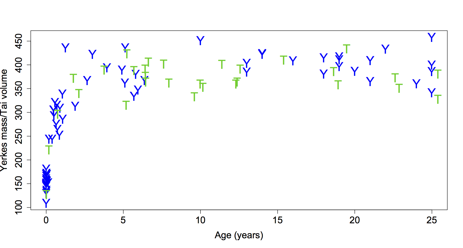
Although I usually present in evolution and fossil-focused sessions, my recent interest in brain growth landed me in a session devoted to Primate Life History this year. The publication of endocranial volumes (ECVs) from wild chimpanzees of known age from Taï Forest (Neubauer et al., 2012) led me to ask whether this cross-sectional sample displays the same pattern of size change as seen in captive chimpanzee brain masses (Herndon et al., 1999). These are unique datasets because precise ages are known for each individual, and this information is generally lacking for most skeletal populations. We therefore have a unique opportunity to estimate patterns and rates of growth, and to compare different populations. Here are the data up to age 25 (the oldest known age of the wild chimps):

fig2 raw data copy

Brain size plotted against age in chimpanzees. Blue Ys are the Yerkes (captive) apes and green Ts are the Taï (wild) chimps. Note that Yerkes data are brain masses while the Taï data are endocranial volumes (ECVs). Mass and volume – as different as apples and oranges, or as oranges and tangerines? Note the relatively high “Y” at 1.25 years, who was omitted from the subsequent analysis.

This is an interesting comparison for a few reasons. First, to the best of my knowledge brain size growth hasn’t been compared between chimp populations (although it has been compared between chimps and bonobos: Durrleman et al., 2012). Second, many studies have found differences in tooth eruption, maturation and skeletal growth and development between wild and captive animals, but again I don’t think this has been examined for brain growth. Finally, and most fundamentally, it’s not clear whether ECV and brain mass follow the same basic pattern of change (brain mass but not ECV is known to decrease at older ages in humans and chimps, but at younger ages…?.

So to first make the datasets comparable, I used published data to examine the relationship between brain mass and ECV in primates, to estimate the likely ECV of the Yerkes brain masses. Two datasets examine adult brain size across different primate species (red and blue in the plot below), and one looks at brain mass and ECV of individuals for a combined sample of gorillas (McFarlin et al., 2013) and seals (Eisert et al., 2013). In short, ECV and brain mass in these datasets give regression slopes not significantly different from 1. One dataset has a negative y-intercept significantly different from 0, meaning that ECV should actually be slightly less than brain mass, but I think this pattern is driven by the really small-brained animals like New World Monkeys).

Untitled

The relationship between endocranial volume and brain mass in primates (and Weddell seals). Solid lines and shaded confidence intervals are given for each regression, and the dashed line represents isometry, or a 1:1 relationship (ECV=brain mass). The rug at the bottom shows the range of the Yerkes masses. Note that the red and black regressions are not significantly different from isometry, while the blue regression is shifted slightly below isometry.

So let’s assume for now that the ECVs of the Yerkes apes are the same as their masses, meaning the two datasets are directly comparable. There are lots of ways to mathematically model growth, and as George Box famously quipped, “All models are wrong, but some are useful.” Here, I wanted to use something that explained the greatest amount of ontogenetic variation in ECV while also levelling off once adult brain size was reached (by 5 years based on visual inspection of the first plot above). This led me to the B-spline. With some tinkering I found that having two knots, one between each 0.1-2.5 and 2.6-5, provided models that fit the data pretty well, and I resampled knot combinations to find the best fit for each dataset. The result:

B-splines describing the relationship between ECV (or brain mass) and age in the TaÏ (green) and Yerkes (blue) data. Although resampling identified different knots for each sample, the regression coefficients are not significantly different.

B-splines describing the relationship between ECV (or brain mass) and age in the TaÏ (green) and Yerkes (blue) data. Note that although the Yerkes line is elevated above the Taï line after 4 years, the confidence intervals (shaded regions) overlap at all ages.

These models fit the data pretty well (r-squared >0.90), and nicely capture the major changes in growth rates. Resampling knot positions reveals best-fit models with different knots for each sample, but otherwise the two models cannot be statistically distinguished from one another: the 95% confidence intervals of both the model coefficients and brain size estimates overlap. So statistical modelling of brain growth in these samples suggests they’re the same, but there are some hints of difference.

Growth rates at each age calculated from the B-spline regressions. Note these are arithmetic velocities and not first derivatives of the growth curves.

Growth rates at each age calculated from the B-spline regressions. Note these are arithmetic velocities and not first derivatives of the growth curves. The dashed horizontal line at 0 indicates the end of brain size growth.

Converting the growth curves to arithmetic velocities we see what accounts for the subtle differences between samples. The velocity plot hints that, in these cross-sectional data, brain size increases rapidly after birth but growth slows down and ends sooner in Taï than among the Yerkes apes. I’m cautious about over-interpreting this difference, since there is great overlap between growth curves, and there is only one Taï newborn compared to about 20 in Yerkes: even just a few more newborns from Taï might reveal greater similarity with Yerkes.

So there you have it, it looks like the wild Taï and captive Yerkes chimps follow basically the same pattern of brain growth, despite living in different environments. Whereas the generally greater stressors in the wild often lead to different patterns of skeletal and dental development in wild vs. captive settings, brain growth appears pretty robust to these environmental differences. That brain growth should be canalized is not too surprising, given the importance of having a well-developed brain for survival and reproduction. But it’s cool to see this theoretical expectation borne out with empirical observations.