Homo habilis just got some long arms to go along with its dexterous hands. In a recent paper in the journal The Anatomical Record, Fred Grine and colleagues describe and analyze some spectacular fossils recovered near the town of Ileret in Kenya, dating to just over 2 million years ago. There were a few different kinds of human-like species inhabiting the planet around this time, but researchers were able to assign these bones to Homo habilis thanks to some chemical clues connecting them to a nearly complete set of teeth found a few meters away. This partial skeleton of a young adult individual is an incredible discovery, connected by clever scientific sleuthing, and provides important information about an early member of the human lineage.
You can see some great photos of these fossils (as well as a fantastic fossil foot of a different individual) in a 2015 press release from the Turkana Basin Institute. A more recent announcement from the Institut Català Paleontologia includes a photo showing the late great Bill Jungers and fossil maven Meave Leakey with the fossils, which helps show the actual size of the bones.
Ann Gibbons’ article about the discovery has a great quote from paleoanthropologist Stephanie Melillo (who discovered the Burtele foot fossil): “If you dressed up a Homo habilis individual in clothes and you saw her walking in the distance, would you do a double take? This study shows us that the answer is YES!”
Artist’s depiction of Homo habilis dressed up in clothes and you see her walking in the distance (image source)
The reason we might react to seeing Homo habilis like Gertie glimpsing E.T., as this skeleton shows, is that this early human had longer arms (especially forearms) than most of us do today. Thickness of the bones also shows that they were probably quite strong as a result of experiencing lots of force from use during life. Long and strong hominin arms are typically interpreted as evidence that these ancient ancestors spent a good deal of time climbing trees.
These features have previously been documented in some of the few other partial skeletons attributed to Homo habilis, as Grine and colleagues note. Indeed, the new article does a deep dive into what is known (and unknown) about the bones and body of Homo habilis, and it also provides a thoughtful review of recent research cautioning against over-interpreting climbing behaviors from fossil remains.
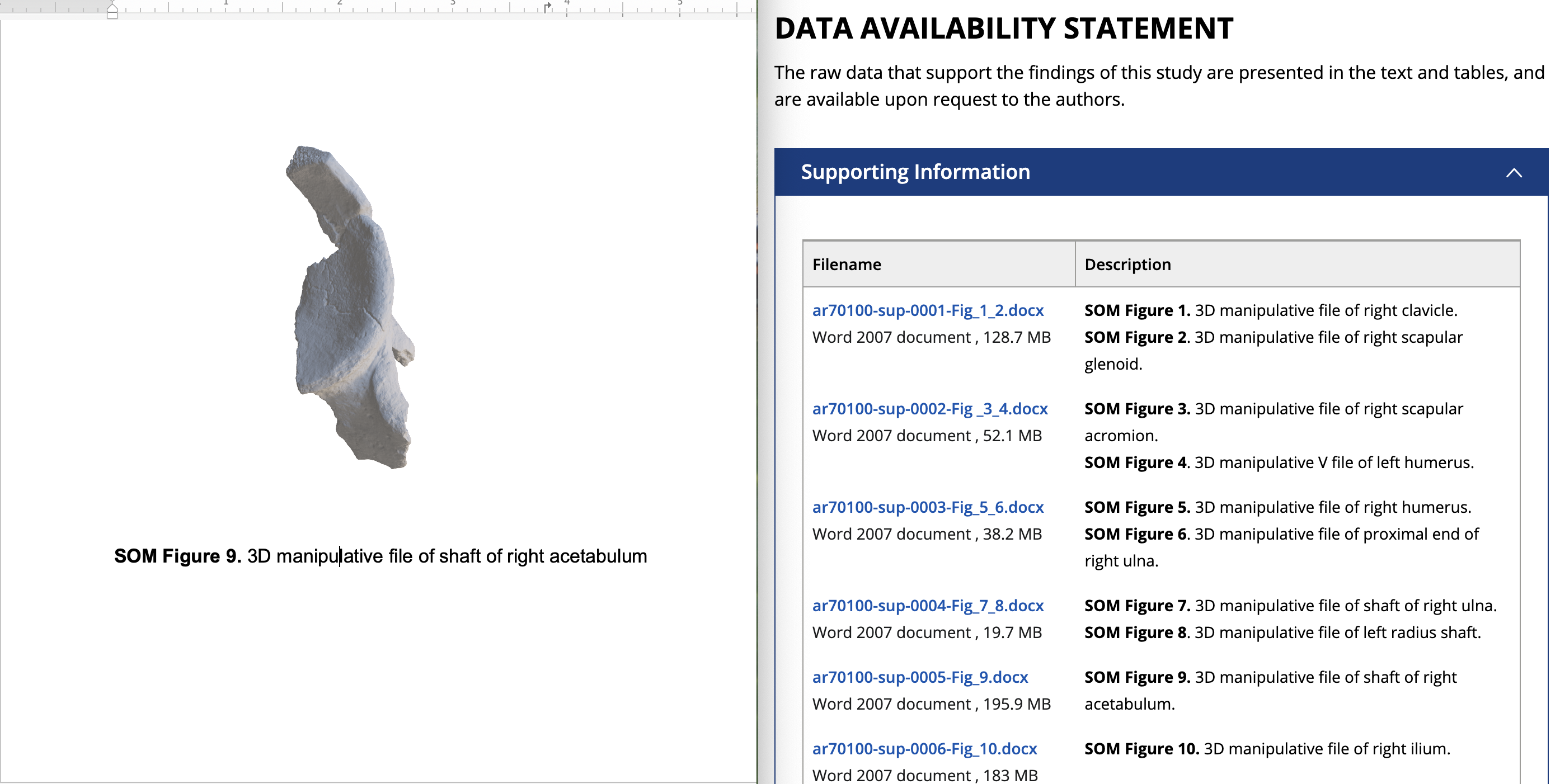
For more fossil fun, the article’s supporting online material includes “3D manipulative files” of the original specimens, so anyone can have a look at the bones in 3D using Microsoft Word:
Dr. Yohannes Haile-Selassie & colleagues just published some amazing fossils from around 3.4 million years ago, that convincingly link an unusual hominin foot fossil to an ancient human called Australopithecus deyiremeda.
In 2012, Haile-Selassie and team reported a foot fossil from Burtele, Ethiopia, revealing a bipedal creature (like a human) but with some grasping ability in the big toe (like all other primates). Then in 2015, the team presented some jaws and teeth from a nearby geological locality in the Burtele region, around which they designated a new hominin species, Australopithecus deyiremeda. The researchers hesitated to allocate the Burtele foot to this new species since they didn’t have similar fossils for comparison between the different fossil localities. But as the scientists have recently reported, jaws and teeth discovered from the foot site, including an incredible juvenile mandible, match those of Au. deyiremeda from the nearby Burtele sites. Now we can put a foot to the name.
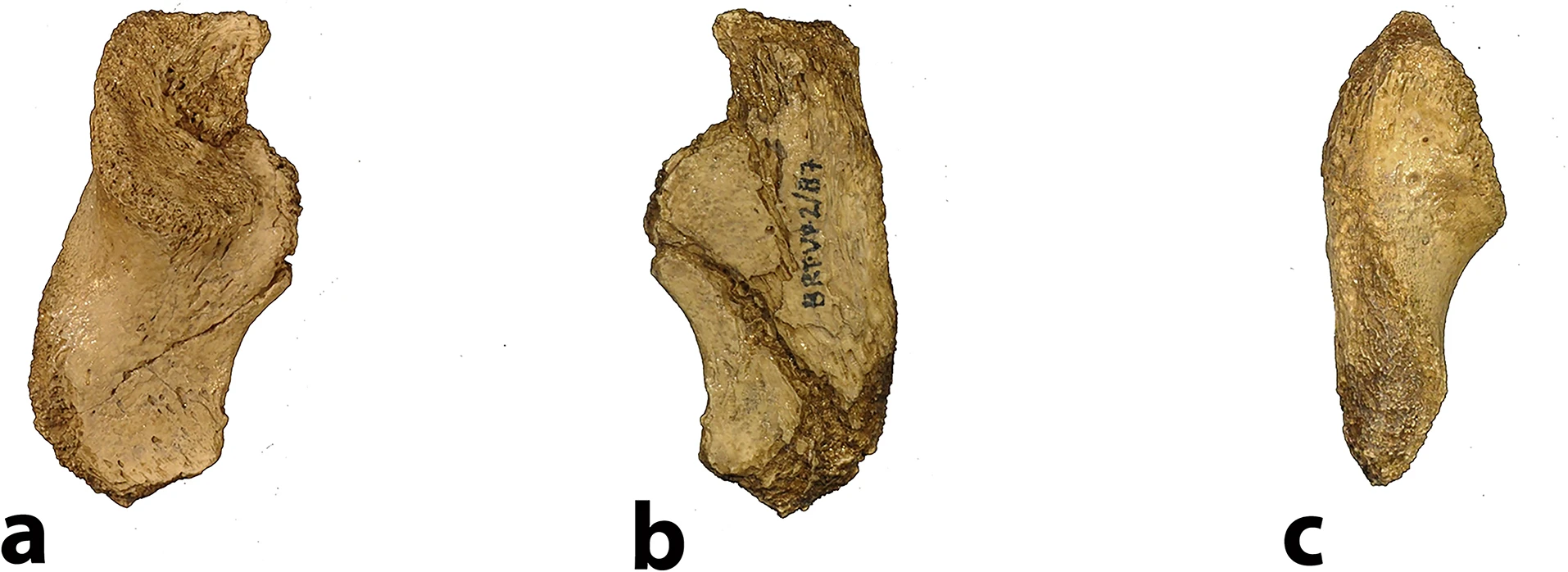
The Burtele fossils help reveal the diversity of early hominins like Australopithecus and the contexts out of which our own genus Homo evolved. What caught my attention hiding among this amazing assemblage was a fossil that only gets a quick mention in the paper—the ischium bone from the hip of a juvenile deyiremeda:
Extended Data Figure 7 from Haile-Selassie et al. (2025). The BRT-VP-2/87 juvenile ischium (from the right side of the body), depicted in side (a), middle (b), and back (c) views.
The fossil, given the catalog number BRT-VP-2/87, represents a different individual from the juvenile jaw mentioned above. It nevertheless provides a great deal of information despite being a small fragment (less than 2 inches long). The authors observe that the body of the ischium that extends beneath the hip joint is quite long, similar to modern apes, fossil Ardipithecus ramidus, and australopiths. This contrasts with the ischium of modern and fossil Homo in which the bone projects less beyond the hip socket:
Right juvenile ischium bones, scaled to similar size and oriented in similar positions. The black line on each depicts the distance from the hip socket margin to the top of the ischial tuberosity (left modified from Scheuer & Black, 2000 Fig. 10.15)
The bottom of the ischium is called the “ischial tuberosity,” and is the attachment surface for the hamstrings muscles. Having a long ischium provides the hamstrings of apes and other arboreal primates with more powerful hip extension—very useful when climbing trees but it also limits how far back the thigh can extend away from the body (Kozma et al., 2018). The shorter ischium of humans, Homo naledi, and other members of our genus may make our hamstrings a little less powerful, but it also helps us fully extend our legs which is crucial to our efficient bipedal walking and running.
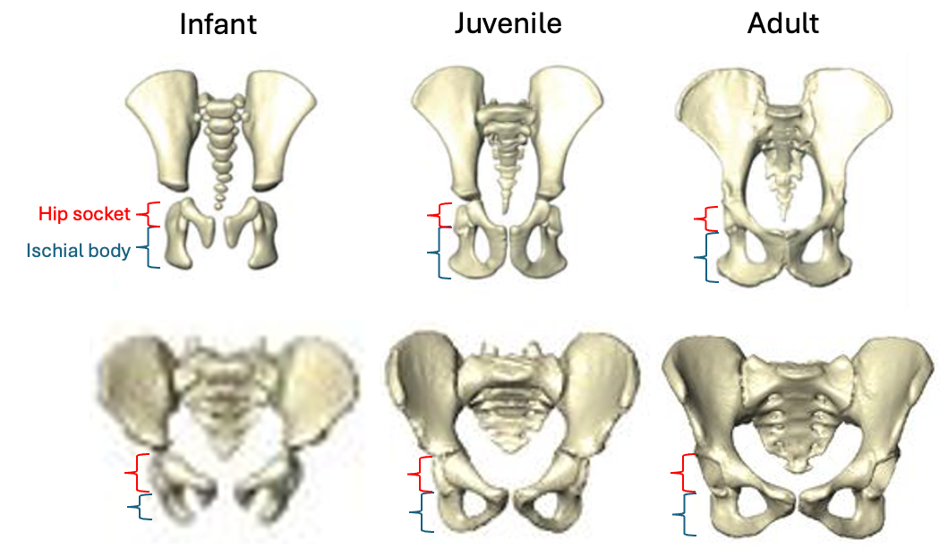
Pelvis growth and development in chimpanzees (top row) and humans (bottom row), all scaled to a similar vertical height. Notice the differences in both the relative length of the ischium (blue bracket) and orientation of the ischial tuberosities between chimps and humans, consistent across the growth period. Images modified from Huseynov et al. (2016 and 2017).
Based on studies of modern humans and other primates, we know that this configuration of bones and muscles is established before birth, so we can be confident that adult Au. deyiremeda would have had a similar anatomy to BRT-VP-2/73, albeit at an unknown, larger size. A hip well adapted for climbing is consistent with the Burtele foot with a grasping big toe.
As Haile-Selassie and colleagues note in the online supplementary information accompanying the paper, only immature fossils allow us to reconstruct the evolution of growth and development. But one of the major challenges of studying immature remains is determining their age or state of maturation, which is critical for understanding how much change occurs between, say, infancy and adulthood. The authors of this study note that the qualitative appearance of the BRT-VP-2/73 hip socket surface is like that of modern humans around 6 years of age, yet the fossil is much smaller and more similar in size to 3 year-old humans. My colleagues and I (2022) faced a similar challenge when analyzing a juvenile Homo naledi hip, and we also relied on qualitative comparisons of how the joint “looks” at different stages of development.
But I think we’re at a point now where we can try to quantify some of these tricky developing surfaces to help place immature fossils more precisely along a timeline of development. For example, Peter Stamos & Tim Weaver (2020) adapted a method for quantifying the topography of teeth, to measure the complex curvature of the developing surface of the knee. If these quantitative methods can distinguish different phases of development in large samples of humans and other primates (e.g., Stamos et al., 2025), they could then be extended to the immature hominin fossil record.
Some cool insights could also be gained by applying older and established methods like landmark-based geometric morphometrics, even on quite fragmentary fossils. This approach could capture the development and orientation of the ischial tuberosity relative to the hip socket surface in fragments like BRT-VP-2/73, MLD 8, and Homo naledi fossils (depicted above) and compared with fossil adults. Researchers have also devised robust ways of quantifying size and shape changes during growth based on modern animals, and using these patterns to then ‘grow’ immature fossils to more developed states, for comparison with actual adult fossils (McNulty et al., 2006). Applying this approach to even just the small fossil sample of ischia described here could tell us a lot about how ancient animals moved at different periods in their lives. Someone just needs to park their ischial tuberosities in a chair and do it!
A growing fossil record of immature hominins, alongside technical advances in quantifying and comparing anatomy, mean that we are ready to learn much more about how our extinct ancestors and cousins grew into competent adults.
Trump and his administration are actively dismantling our economy and democratic institutions. One of the most recent parts of this assault is an executive order issued last week, “Restoring Truth and Sanity to American History.” The title itself is Orwellian doublespeak since the order describes the rejection of truth and science, while it in fact aims to whitewash American history.
An entire section of the order is devoted to, “Saving our Smithsonian” Institution, the national complex of museums, education outreach programs, research facilities, and a large Zoo. The order singles out an exhibit at the American Art Museum because it, “promotes the view that race is not a biological reality but a social construct … ‘a human invention.'”
As noted in the New York Times, the exhibit displays many quotations from the Statement on Race & Racism published by the American Association of Biological Anthropologists a few years ago. The statement explains, “Humans are not divided biologically into distinct continental types or racial genetic clusters,” which I think gets at the fundamental misconception most Americans have about race. Whether uninformed or outright racist and malicious, many people conceive of race as an invisible, unchanging essence that determines an individual’s capacities and behaviors. In the olden days race was thought of as ancestral and ‘in the blood,’ but in the genomic age people began attributing racial essence to DNA. All of these biological data—from blood to whole genomes—for at least the past fifty fucking years have shown that, again, “Humans are not divided biologically into distinct continental types or racial genetic clusters.”
Now, some folks who call themselves “race realists” (you can’t spell “race realist” without “racist”) might point to scientific research about human genetic variation with graphs showing humans partitioned into statistically-inferred clusters corresponding roughly with geography. The problem that tends to arise from here is the over-interpretation this within-species variation. As Lewontin showed back in 1972, and subsequent studies have consistently confirmed with more and more data, the amount of genetic variation that distinguishes different populations is but a small proportion (less than 15%) of the overall variation within our species. What’s more, because this variation is scattered throughout all of our DNA, most of it should be “neutral” with regard to evolution, with little or no effect on how likely an individual is to survive or reproduce. Simply put, humans across the planet are more genetically similar than different, and the limited genetic differences between populations probably doesn’t really influence how they behave or what they are capable of. Even though geneticists have argued this for years, many Americans are still quick to over-interpret the biological significance of these minuscule genetic differences, often tragically so.
To the contrary, race as many people think of it today is a recent historical concept – a “Fatal Invention” as Dr. Dorothy Roberts explains in her 2012 book. This is the consensus among experts in both the natural and social sciences. Yet Trump’s executive order specifically rejects this well established knowledge that race is in fact “a human invention,” as the order quotes from the Smithsonian art exhibit. This is one of the many purposes of rejecting the science and claiming that race is a biological reality — it serves to naturalize social differences and social inequality. If you maintain that people’s qualities are genetically determined and that groups differ fundamentally in their inherited genetics, then you have justification for avoiding social interventions to racial (and other kinds of social) inequality. As Dr. Michael Blakey explained back in 1999, “Race is essentially a means of defining ethnic and social status groups as biological entities. … In a racist or White Supremacist society, such as the United States, this … will often become the basis for decisions about the allocation of social resources and the solutions to social problems.”
Trump and Musk are both known to harbor unscientific and racist views about genetics, and both have been associated with far right and often white supremacist groups. The recent executive order claims that by communicating the actual science of human variation and the history of racism in this country, the Smithsonian is “under the influence of a divisive, race-centered ideology.” But with this administration, every accusation is a confession. They are actively dismantling our institutions and efforts that aim to address and repair the damage from centuries of racism, in order to advance their own white supremacist agenda (see for example here, here, and here).
Gibbons are sometimes referred to as “lesser apes” since they’re the smaller-bodied cousins of “great apes” like us humans, chimpanzees, gorillas, and orangutans. But what they lack in body mass they make up for in taxonomic diversity, with roughly 20 species distributed across four genus groups (Kim et al., 2011). And while male great apes (except humans) have large canine teeth, both sexes in gibbons have large maxillary canines — flashy weaponry for defending territory.
Pointy canine teeth peeking out from the upper and lower jaws of an adult female gibbon cared for at the International Primate Protection League (source)
My research has generally focused on brains and growth throughout human evolution, but I started looking at gibbons a few years ago when the COVID-19 pandemic put research travel on hold. Inspired by Julia Zichello’s 2018 article about gibbon models for understanding hominin evolution and appreciating that “overlooked small apes need more attention,” I had the opportunity to CT scan a unique skeletal collection of white-handed gibbons (Hylobates lar), which was sadly harvested from the forests of Thailand back in the late 1930s. Previous research on skull growth in gibbons has mostly used small samples compiled from different species (and sometimes even different genera). In contrast, this CT dataset includes many individuals at each stage of maturation from late infancy through adulthood, effectively representing a single population at a point in time. So with this larger cross-sectional sample of a single species, we can better understand how gibbon brains and faces grow. And because permanent teeth form in a long, continuous sequence throughout the growth period, an individual’s state of dental development can serve as a marker of where they are along the maturation process.
In a paper hot off the press, Julia Boughner and I analyzed dental development in this unique sample (article here). One of the coolest things we found was that gibbons’ large upper canine teeth are among the first to begin but last to finish tooth formation. In fact, the large canines growing inside relatively small faces may inhibit growth of one of the neighboring incisor teeth until the face has grown to create enough space for it. And while most teeth developing within the jaw begin emerging into the mouth once there’s enough room for them, gibbons’ gargantuan upper canines are forced out of hiding as they outgrow their bony crypts (check out the right-most jaw in the second row below).
Cross-sectional representation of tooth formation in white-handed gibbons, starting with the youngest in the top left and ending with the oldest in the bottom right. The first permanent tooth to form and emerge, M1, is highlighted along with the canine “C.”
In addition to characterizing ‘normal’ dental development, we also observed several developmental anomalies and pathologies in the sample. Our observations corroborate previous research showing that tooth formation generally proceeds ‘as scheduled’ despite various other disturbances to development.
It remains to be seen whether early development of the canine at the cost of delayed incisor formation is a pattern unique among all the apes, since most other studies of ape tooth formation have examined the lower jaw while our study focused on the upper jaws. But the canine-incisor tradeoff that we identified sets the stage for subsequent study of skull growth in this sample, as it highlights the many factors and functions that must be coordinated during growth.
While we have several projects planned with this unique dataset, we have also published the tooth formation data that we analyzed, and the original micro-CT scans themselves will be published to the online repository Morphosource.org soon, once a few more projects are finished.
For the first time in many years, I’m offering a new advanced undergrad seminar here at Vassar. When I arrived here 8 years ago, I was mainly thinking about Homo naledi and ontogeny, so those were the foci of my seminars. But my research has begun looking more at brain evolution and especially the evidence from fossil endocasts, and there is a lot of literature I need to catch up on.
So I’ve invited students along for this brainstorm, using the question “Is the human brain special?” as a starting point to learn about how the beautifully congealed soup sloshing around inside our skull makes us such quirky animals. In the first half of the semester we’ll read up on brain anatomy and structure, and students will use some of the fossil endocast data I’ve accrued over the years to learn more about a given brain region and extinct hominin. In the second half of the semester we’ll read about the brains, behavior, and endocast fossils of very distant relatives — invertebrates, birds, whales, and dogs — that have been celebrated for their own ‘advanced intelligence.’ We’ll also read about how the evolution of our brains may have predisposed us to certain conditions like addiction and Alzheimer’s, and how brain science has been exploited toward racist and sexist ends (increasingly relevant in America today, sadly).
It will be a lot of work (I’m a very slow, distractible reader) but I’m excited to delve into this literature and see what insights our super sharp students here at Vassar come up with in discussions and projects. The course syllabus (ANTH 323) is available on my Teaching page — I’d be keen to hear suggestions for readings and assignments from folks who know more about brains than I do!
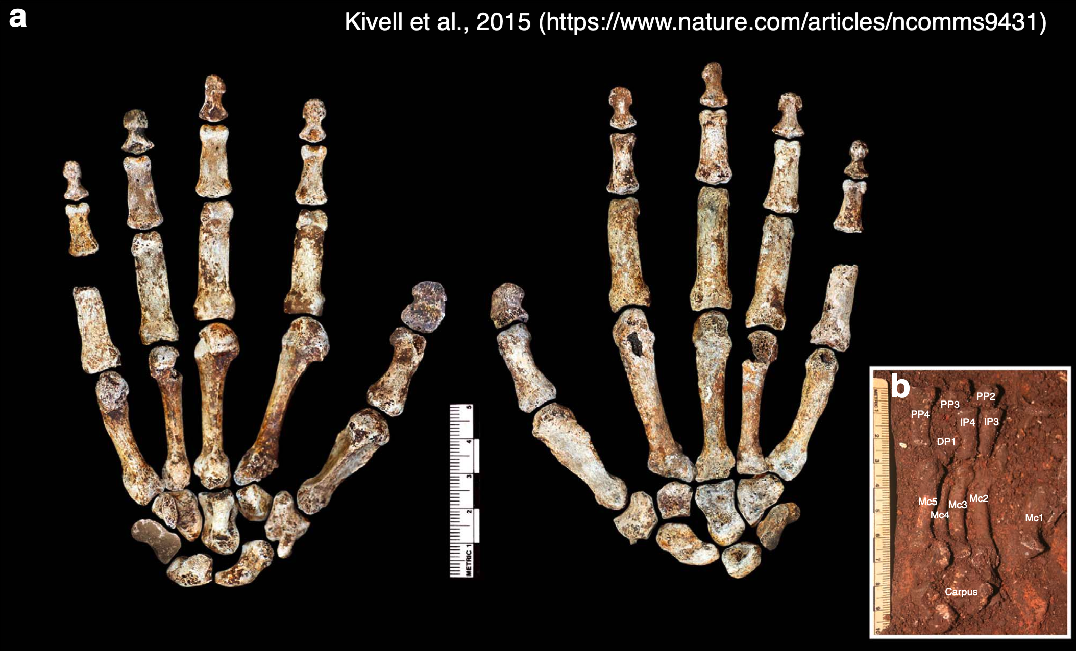
Homo naledi is one of my favorite extinct humans, in part because its impressive fossil record provides rare insights into patterns and process of growth and development. When researchers began recovering naledi fossils from Rising Star Cave 10 years ago, one of the coolest finds was this nearly complete hand skeleton. The individual bones were still articulated practically as they were in life so we know which bones belong to which fingers, allowing us grasp how dextrous this ancient human was. And since finger proportions are established before birth during embryonic development, we can see if Homo naledi bodies were assembled in ways more like us or other apes.
The “Hand 1” skeleton of Homo naledi, adapted from a figure by Kivell and colleagues (2015). Left shows the palm-side view while the middle shows the back of the hand. The inset (b) shows many of the palm and finger bones as they were found in situ in Rising Star Cave.
In a paper hot off the press (here), I teamed up with Dr. Tracy Kivell to analyze finger lengths of Homo naledi from the perspective of developmental biology. On the one hand, repeating structures such as teeth or the bones of a finger must be coordinated in their development, and scientists way smarter than me have come up with mathematical models predicting the relative sizes of these structures (for instance, teeth, digits, and more). On the other hand, the relative lengths of the second and fourth digits (pointer and ring fingers, respectively) are influenced by exposure to sex hormones during a narrow window in embryonic development: this ‘digit ratio’ tends to differ between mammalian males and females, and between primate species with different social systems.
So, Tracy and I examined the lengths of the three bones within the second digit (PP2, IP2, DP2) and of the first segment of the second and fourth digits (2P:4P) in Homo naledi, compared to published data for living and fossil primates (here and here). What did we find out?
Summary of our paper showing the finger segments analyzed (left), and graphs of the main results (right). The position of Homo naledi is highlighted by the blue star in each graph.
The first graph above compares the relative length of the first and last segments of the pointer finger across humans, apes, and fossil species. The dashed line shows where the data points are predicted to fall based on a theoretical model of development. There is a general separation between humans and the apes reflecting the fact that humans have a relatively long distal segment, which is important for precise grips when manipulating small objects. Fossil apes from millions of years ago and the 4.4 million year old hominin Ardipithecus are more like apes, while Homo naledi and more recent hominins are more like modern humans. Because both humans and apes fall close to the model predictions, this means the theoretical model does a good job of explaining how fingers develop. Because humans and apes differ from one another, this suggests a subtle ‘tweak’ to embryonic development may underlie the evolution of a precision grip in the human lineage, and that it occurred between the appearance of Ardipithecus and Homo.
The second graph compares the ‘digit ratio’ of the pointer and ring fingers from a handful of fossils with published ratios for humans and the other apes. Importantly, the digit ratio is high in gibbons (Hylobates) which usually form monogamous pair bonds, while the great apes (Pongo, Gorilla, Pan) are characterized by greater aggression and mating competition and have correspondingly lower digit ratios. Ever the bad primates, humans fall in between these two extremes. Most fossil apes and hominins have digit ratios within the range of overlap between the ape and human ratios, but Homo naledi has the highest ratio of all fossil hominins known, just above the human average. It has previously been suggested that humans’ higher ratio compared to earlier hominins may result from natural selection favoring less aggression and more cooperation recently in our evolution. If we can really extrapolate from digit proportions to behavior, this could mean Homo naledi was also less aggressive. This is consistent with the absence of healed skull fractures in the vast cranial sample (such skull injuries are common in much of the rest of the human fossil record).
You can see the amazing articulated Homo naledi hand skeleton for yourself on Morphosource. Its completeness reveals how handy Homo naledi was 300,000 years ago, and it can even shed light on the evolution of growth and development (and possibly social behavior) in the human lineage.
In the Summer of 2019 I worked with some great Vassar undergrads to make virtual endocasts and generate new brain size estimates for the Neandertals from the site of Krapina, which we then published in 2021 (discussed in this blog post). The virtual approach to endocast reconstruction uses 3D landmark-based geometric morphometrics methods, and so in the spirit of open science we also published all the landmark data used for the study (as well as a bunch of other fossil human brain size estimates) in the Zenodo repository (here).
Neandertal fossil specimens Krapina 3 (purple/green) and Krapina 6 (yellow/red) with preserved landmarks and virtually reconstructed endocasts.
Something major and global happened around that time — who can even remember what? — and so I never got around to posting R code to accompany the study. So, I’ve finally gotten around to adding some very basic code to the Zenodo entry (better late than never). The code simply reads in the landmarks, estimates missing data for fossils, and does some very basic shape analysis and visualization. It’s doesn’t get into all the nuts and bolts of our study, but it should be enough to help folks check our data or get started with shape analysis in R.
R code includes ways to visualize the landmark data. Left: Principal components analysis graph of endocast shape for humans (red) and Neandertals (blue). Right: Triangle meshes of the average human and Neandertal endocast shapes, viewed from the right, bottom, and back.
Original article Cofran Z, Boone M, Petticord M. 2021. Virtually estimated endocranial volumes of the Krapina Neandertals. American Journal of Physical Anthropology 174: 117–128. (link)
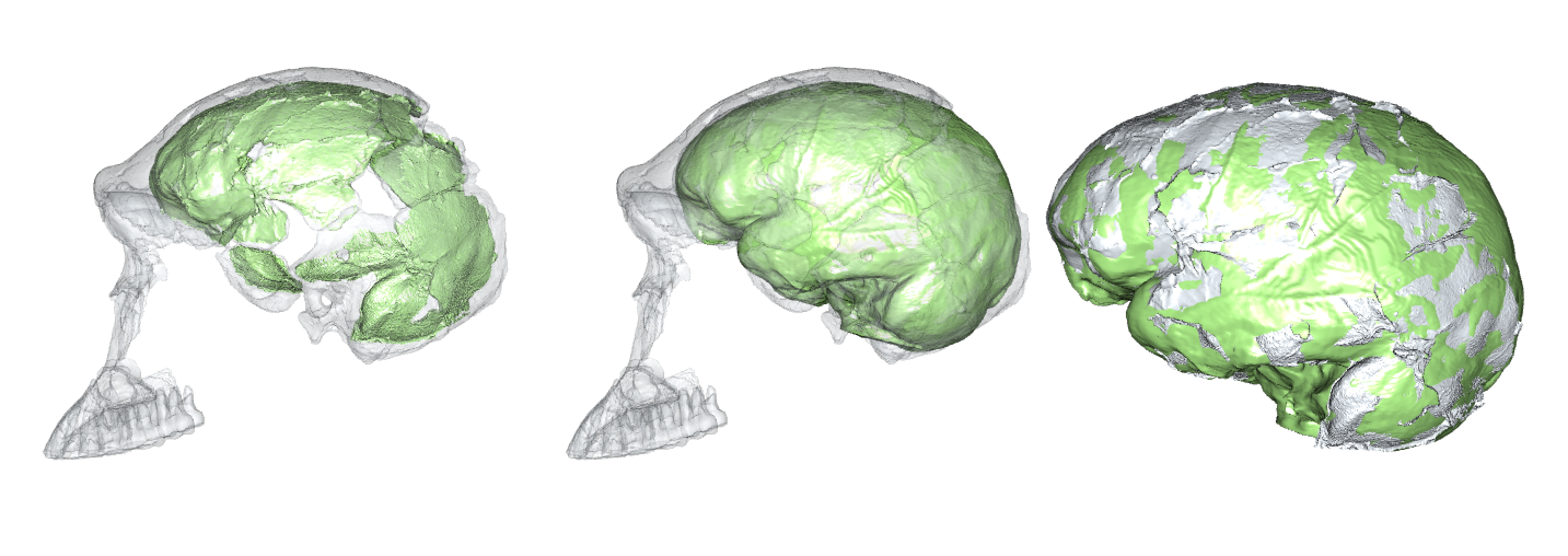
What makes the human brain special, and how did it change throughout our evolutionary history? One way to answer this question by comparing actual brains or MRI scans of living animals. But only fossils can show what changed and when over the past several million years, and sadly brains are basically an elaborately congealed soup that doesn’t stay fresh upon death, so they never fossilize (well, almost never). Happily, though, bones can preserve for millions of years, and they are literally molded by their soft and squishy surroundings. As the brain grows, it pushes outward against the inner surface of the skull, which can save the scars of the submerged cerebrum: nerds like me call these impressions an “endocast.”
Endocasts of Homo naledi (pink) and Homo erectus (yellow). Fossils are viewed from the left side and are variably preserved.
Nicole Labra and Antoine Balzeau have led a cool study, hot off the press, examining what such endocasts can tell us about the underlying brain anatomy. Importantly, they show how difficult it is to clearly and consistently identify many brainy boundaries. This is very salient in “paleoneurology,” the study of brain evolution especially based off endocasts: the problem probably best illustrated by the nearly century-long debate about the natural endcoast of the “Taung child” fossil (Australopithecus africanus).
Labra & colleagues used a clever approach to address this paleontological and epistemological problem. They first generated an endocast directly associated with its brain from an MRI scan of a living human, allowing them see precisely where specific brain grooves (“sulci”) lay relative to the endocast surface. They then asked a bunch of researchers—myself included—to try to identify sulci on the endocast, and then looked at how our responses compared to both one another’s and to the actual, known sulcus positions.
Figure 1 from Labra et al. (in press) showing how the brain and endocast were obtained and analyzed.
Their analysis showed that we varied quite a bit in our identifications on the endocast. As Emiliano Bruner (who also participated) discusses in his blog post, we tended to identify the stronger impressions toward the bottom and sides of the endocast better and more consistently. Some of this variability and uncertainty among researchers is due to the faintness and incompleteness of many brain impressions, and some due to biased expectations about where a given sulcus “should” be based on our previous experiences and published references.
When Antoine Balzeau first contacted me about this project, I was just beginning to dabble in paleoneurology, learning some brain anatomy for the first time for a description of an old Australopithecus endocast called “MLD 3.” I initially thought MLD 3 would be a quick and simple study—boy was I spectacularly disappointed!
Figure 3 from Cofran et al. 2023, comparing two different chimpanzee brains, and two corresponding interpretations of the MLD 3 endocast.
Probably reflecting observer bias and desire for definitive results, we initially interpreted the endocast impressions on MLD 3 as representing a ‘human-like’ anatomy that is super rare in living chimpanzees (namely the “LS” depicted in the right half of the figure above). The researchers who peer-reviewed the first draft of our paper, though, suggested we be more cautious in our interpretations; one reviewer outright disagreed with us in support of a more ‘ape-like’ interpretation (left half of the figure above). The review process alone underscored the subjectivity and uncertainty in analyzing endocasts. In the end we presented both interpretations, and I honestly don’t know which (if either) is most likely to be correct. So the study by Labra and colleagues provides a nice empirical illustration of this cranial conundrum.
Fortunately, researchers are developing methods to help identify brain structures on endocasts. Amélie Beaudet, Jean Dumoncel, and Edwin de Jager among others have done some really impressive work looking at variability in both brains (for instance here) and endocasts (for instance here). By using computer-based 3D data and methods, these researchers have shown where many brain sulci tend to be located (see here). By developing a better understanding of variation in where sulci sit on an endocast, we can have a better idea of which sulci might be represented on fossil endocasts, which in turn can tell us about the brains of our extinct relatives. Edwin and Amélie presented a very cool new analysis of Australopithecus/Paranthropus boisei endocasts, building off this digital approach, at the recent ESHE conference. And as noted in our MLD 3 paper, I think machine learning and other ‘artificial intelligence’ approaches could also help us identify ambiguous features from frustrating fossil fragments.
I’m working on a project analyzing infant remains of Homo naledi, a species of human that lived in South Africa around 300,000 years ago. In order to paint a full picture of infancy in this species, we need to estimate how big (or small) naledi newborns were. But without fossil neonates that could provide direct evidence of body size at birth, this is a tricky task.
Ideally, we could simply use adult body size estimates for Homo naledi to predict its body size at birth, using the scaling relationship in other primates as a guide. For example, using an average adult body size of 44 kg for Homo naledi (Garvin et al., 2017) yields an estimated newborn size of around 1.5 kg, based on published primate dataset (Barton and Cappellini, 2011). But this approach necessarily overlooks variation within each species, not to mention variation and uncertainty in Homo naledi adult size. In addition, the 95% prediction interval for this estimate ranges from under 1 kg (smaller than an average baboon baby) to almost as large as a human neonate.
Primate body size scaling (Barton & Cappellini, 2011). The black line is the regression for catarrhines (purple squares and blue circles), and the shaded grey area is the 95% prediction interval for newborns at a given adult catarrhine size.
And this gets at the other issue with the regression-based approach to estimating newborn body size in fossil hominins: humans are bad at being primates in some ways, as illustrated here by the fact that we don’t fit the newborn-adult body size relationship that characterizes other catarrhines (apes and monkeys of Africa and Eurasia).
Humans give birth to collosal kids. In contrast, gorillas are the largest living primates as adults, but their newborns are only a little over half the size of human neonates. Why do we have such giant babies? The most proximate reason is that humans are born with adult-ape-sized brains and quite a bit of baby fat as far as mammals go (Kuzawa, 1998). This tells us how babies are big, but it still begs the ultimate question of why—an enduring puzzle that you may have read about in the New York Times last week.
In order to land on a reasonable estimate of newborn body size in extinct humans, we need to figure out when evolution blew up the kid. Unfortunately, the only fossil hominin neonates are two Neandertals from France and Russia dating to under 100,000 years ago—pretty remarkable, but they don’t necessarily tell us about earlier species like Homo naledi.
My colleague Jerry Desilva (2011) worked out a potential solution to this conundrum. He argued that one could work from adult brain size to newborn body size through the following steps. First, in contrast to newborn-adult body size scaling, humans are good catarrhines when it comes to newborn-adult brain size scaling. This means that we can reasonably estimate newborn brain size based on adult brain sizes, which are aplenty in the human fossil record. Second, humans and many other primate newborns have brains roughly 12% of their overall body mass, while the great ape newborns stand out with brains around 10% of their adult size. Putting these two pieces together, one could estimate newborn body size: Adult brain ➡️ newborn brain ➡️ 10–12% newborn body size
DeSilva showed that regardless of whether you use an ape or human model of newborn brain/body size, hominin babies from Australopithecus afarensis 3 million years ago onward were probably large relative to maternal body size, estimated independently using skeletal remains. It’s a bit of a tortuous approach to estimating body size at birth, but the assumptions are reasonable and it’s probably the best way to figure out this important life history variable given the fossil evidence. What does this mean for Homo naledi?
Virtual reconstruction of brain size and shape of the Homo naledi cranium “Neo” (work in progress). At 610 cm3, this is the largest and most complete Homo naledi endocast.
There are a few reliable adult brain size estimates for naledi, ranging from 465–610 cm3 (Berger et al., 2015; Garvin et al., 2017; Hawks et al., 2017), which based on catarrhine scaling would predict newborn brain size of around 170–210 cm3 (DeSilva and Lesnik, 2008). These brain sizes would then predict newborn body sizes of around 1.4–2.1 kg: the smol estimate is based on the smallest naledi adult brain size and a human model of newborn brain/body size; the chonk estimate is based on the largest naledi brain size and an ape brain/body model (pinkish stars in the boxplot below, left).
Boxplots of newborn body size in great apes. Gorilla, Chimpanzee, and Bonobo data from the Primate Aging Database(Kemnitz, 2019).
So, did Homo naledi have big babies? On the one hand, no: these 1.4–2.1 kg naledi newborns are outside the human range, and within the range of living great apes.
On the other hand, maybe Homo naledi babies were relatively large, though this depends on the size of Homo naledi adults. Recall from earlier that Garvin and colleagues arrived at an average estimated adult size of 44.2 kg. But this is an average of estimates for 20 separate naledi fossils, and each of these estimates has its own range of uncertainty. Garvin and team reported that the extremes of the prediction intervals for these estimates ranged from 28–62 kg. The second boxplot above shows newborn size relative to the adult average (sexes combined) for each species: for naledi, the six labels compare the smol and large newborn sizes (1.4 and 2.1 kg) with the adult average and extremes (28, 44, and 62 kg). Assuming the ‘true’ naledi sizes are somewhere in the middle of the range of estimates, naledi likely gave birth to babies 3–5% of adult body size, somewhat ‘intermediate’ between chimpanzees and humans (and bonobos…?) and similar to what DeSilva found for other hominins.
This is just a preliminary look at infancy in Homo naledi. There is a lot of uncertainty in these size estimates, but we should still be able to make some interesting inferences about growth and life history in our extinct evolutionary cousin.
REFERENCES
Barton, R. A., & Capellini, I. (2011). Maternal investment, life histories, and the costs of brain growth in mammals. Proceedings of the National Academy of Sciences, 108(15), 6169–6174. https://doi.org/10.1073/pnas.1019140108
Berger, L. R., Hawks, J., de Ruiter, D. J., Churchill, S. E., Schmid, P., Delezene, L. K., … Zipfel, B. (2015). Homo naledi, a new species of the genus Homo from the Dinaledi Chamber, South Africa. ELife, 4, e09560. https://doi.org/10.7554/eLife.09560
DeSilva, J. M. (2011). A shift toward birthing relatively large infants early in human evolution. Proceedings of the National Academy of Sciences, 108(3), 1022–1027. https://doi.org/10.1073/pnas.1003865108
DeSilva, J. M., & Lesnik, J. J. (2008). Brain size at birth throughout human evolution: A new method for estimating neonatal brain size in hominins. Journal of Human Evolution, 55(6), 1064–1074. https://doi.org/10.1016/j.jhevol.2008.07.008
Garvin, H. M., Elliott, M. C., Delezene, L. K., Hawks, J., Churchill, S. E., Berger, L. R., & Holliday, T. W. (2017). Body size, brain size, and sexual dimorphism in Homo naledi from the Dinaledi Chamber. Journal of Human Evolution, 111, 119–138. https://doi.org/10.1016/j.jhevol.2017.06.010
Hawks, J., Elliott, M., Schmid, P., Churchill, S. E., Ruiter, D. J. de, Roberts, E. M., … Berger, L. R. (2017). New fossil remains of Homo naledi from the Lesedi Chamber, South Africa. ELife, 6, e24232. https://doi.org/10.7554/eLife.24232
Kuzawa, C. W. (1998). Adipose tissue in human infancy and childhood: An evolutionary perspective. American Journal of Physical Anthropology, 107(S27), 177–209. https://doi.org/10.1002/(SICI)1096-8644(1998)107:27+<177::AID-AJPA7>3.0.CO;2-B
Each year in my intro bio-anthro class, we start the course by asking how our brains contribute to making us humans such quirky animals. Our first lab assignment in the class uses 3D models of brain endocasts, to ask whether modern human and fossil hominin brains are merely primate brains scaled up to a larger size. In the Before Times, students downloaded 3D meshes that I had made, and study and measure them with the open-source software Meshlab. But since the pandemic has forced everyone onto their own personal computers, I made the activity all online, to minimize issues arising from unequal access to computing resources. And since it’s all online, I may as well make it available to everyone in case it’s useful for other people’s teaching.
The lab involves taking measurements on 3D models on Sketchfab using their handy measurement tool, and entering the data into a Google Sheets table, which then automatically creates graphs, examines the scaling relationship between brain size (endocranial volume, ECV) and endocast measurements, and makes predictions about humans and fossil hominins based off the primate scaling relationship. Here’s the quick walk-through:
Go to the “Data sources” tab in the Google Sheet, follow the link to the Sketchfab Measurement Tool, and copy the link to the endocast you want to study (3D models can only be accessed with the specific links).
Following the endocast Sketchfab link (column D) will bring you to a page with the 3D endocast, as well as some information about how the endocast was created and includes its overall brain size (ECV in cubic cm). Pasting the link when prompted in the Measurement Tool page will allow you to load, view, and take linear measurements on the endocast.
Hylobates lar endocast, measuring cerebral hemisphere length between the green and red dots.
Sketchfab makes it quite easy to take simple linear measurements, by simply clicking where you want to place the start and end points. The 3D models of the endocasts are all properly scaled, and so all measurements that appear in the window are in millimeters.
The assignment specifies three simple measurements for students to take on each endocast (length, width, and height). In addition, students get to propose a measurement for the size of the prefrontal cortex, since our accompanying reading (Schoenemann, 2006) explains that it is debated whether the human prefrontal is disproportionately enlarged. All measurements are then entered into the Google Sheet — I wanted students to manually enter the ECV for each endocast, to help them appreciate the overall brain size differences in this virtual dataset (size and scale are often lost when you have to look at everything on the same-sized 2D screen).
Feel free to use or adapt this assignment for your own classes. The assignment instructions can be found here, and the data recording sheet (with links to endocast 3D models) can be found here — these are Google documents that are visible, but you can save and edit them by either downloading them or making a copy to open in Docs or Sheets.