When everyone’s losing it.
Last week, I discussed the implications of the Gona hominin pelvis for body size and body size variation in Homo erectus. One of the bajillion things I have been working on since this post is elaborating on this analysis to write up, so stay tuned for more developments!
Now, when we compared the gross size of the hip joint between fossil Homo and living apes (based on the femur head in most specimens but the acetabulum in Gona and a few other fossils), the range of variation in Homo-including-Gona was generally elevated above variation seen in all living great apes. This is impressive, since orangutans and gorillas show a great range of variation due sexual dimorphism (normal differences between females and males). However, I noted that the specimens I used were unsexed, and so the resampling strategy used to quantify variation within a species – randomly selecting two specimens and taking the ratio of the larger to smaller – probably underestimated sexual dimorphism.
Shortly after I posted this, Dr. Herman Pontzer twitterated me to point out he has made lots of skeletal data freely available on his website (a tremendous resource). The ape and human data I used for last week’s post did not have sexes (my colleague has since sent me that information), but Pontzer’s data are sexed (no, not “sext“). So, I modified and reran the original resampling analysis using the Pontzer data, and it nicely illustrates the difference between using a max/min vs. male/female ratio to compare variation:

Hip joint size variation in living African apes (left and right) compared with fossil humans (genus Homo older than 1 mya, center). Each plot is scaled to show the same y-axis range. On the left are ratios of max/min from resampled pairs from each species (sex not taken into account). On the right are ratios of male/female from resampled pairs from each species. The red stars on this plot are the medians for max/min ratios (the thick black bars in the left plot). The center plot shows ratios of Homo/Gona.
The left plot shows resampled ratios of max/min in humans, chimpanzees and gorillas, while the right shows ratios of male/female in these species. If no assumption is made about a specimen’s sex (left plot), it is possible to resample a pair of the same sex, and so it is likelier to sample two individuals similar in size. Note that the ratio of max/min can never be less than 1. However, if sex is taken into account (right plot), we see two key differences. First, because of size overlap between males and females in humans and chimpanzees, ratios can fall below 1. Adult gorilla males are much larger than females, and so the ratio is never as low as 1 (minimum=1.08). Second, in more dimorphic species, the male/female ratio is elevated above the max/min ratio (red stars in the right plot). In chimpanzees, the median male/female ratio is actually just barely lower than the median max/min ratio. If you want numbers: the median max/min ratios for humans, chimpanzees and gorillas are 1.09, 1.06 and 1.16, respectively. The corresponding median male/female ratios are 1.15, 1.06 and 1.25.
Regarding the fossils, if we assume that Gona is female and all other ≥1 mya Homo hips are male, the range of hip size variation can be found within the gorilla range, and less often in the human range.
But the story doesn’t end here. One thing I’ve considered for the full analysis (and as Pontzer also pointed out on Twitter) is that the relationship between hip joint size and body weight is not the same between humans and apes. As bipeds, we humans place all our upper body weight on our hips; apes aren’t bipedal and so relatively less of their weight is transmitted through this joint. As a result, human hip joint size increases faster with increasing body mass than it does in apes.
So for next installment in this fossil saga, I’ll consider body mass variation estimated from hip joint size. Based on known hip-body size relationships in humans vs. apes, we can predict that male/female variation in humans and fossil hominins will be relatively higher than the ratios presented here – will this put fossil Homo-includng-Gona outside the gorilla range of variation? Stay tuned to find out!
UPDATE: sadly, the KUPRI Digital Morphology Museum website, which was the basis for this activity, is no longer online 😦 If I can find a comparable resource I will be sure to update this post.
The focus of my human evolution class the past few weeks has been uncovering the earliest human ancestors. The main adaptation distinguishing our first forebears from other animals is walking on two legs (“bipedalism”), so researchers try to identify features reflective of bipedalism in fossils over 4 million years ago. But this isn’t so easy – not all fossils will tell us how an animal walked around, and even with the right bones, it’s not always clear what the earliest bipeds “should” look like. Take the case of Ardipithecus kadabba: there are a handful of seemingly nondescript fossils (below) from a number of Ethiopian sites dating 5.2-5.8 million years ago. Can we really tell if this species was bipedal? LET YOUR STUDENTS DO SCIENCE TO DECIDE FOR THEMSELVES!

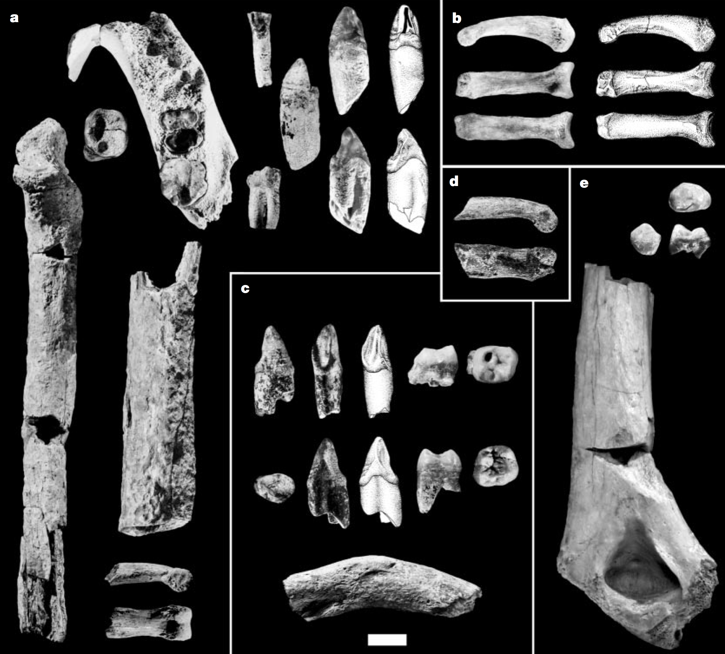
Can you spot a biped? Ardipithecus kadabba fossils. Scale bar is 1 cm (Fig. 1 from Haile-Selassie, 2001).
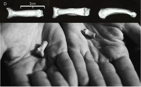
In the jumble of fragments pictured above, the key bone possibly revealing a bipedal animal is in square b, a toe bone shown in several views. This is a fourth proximal pedal phalanx (PPP4), where a wedding ring would sit if people put rings on their feet instead of their hands. Ew. Anyway, here’s closer view, from the Ar. kadabba monograph (Haile-Selassie and WoldeGabriel, 2009):

Top: AME-VP 1/71, the sciencey name of the toe bone in question. The proximal end (toward the foot) is to the left and the distal end (toward the tip of the toe), is to the right. Bottom: Lookit how tiny it is! Modified from plates 7.8 and 7.21 in the monograph.
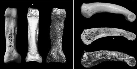
Although absolutely small, the kadabba PPP4 is relatively long, narrow and curved, like an ape’s and unlike a human’s. Haile-Selassie and colleagues (monograph chapter) compared this fossil with chimpanzee and the bipedal Australopithecus afarensis‘s PPP4s (below I have scaled them to the same length). As you can see, kadabba and the chimp are fairly narrow compared to the stout afarensis toe, although they are all curved:

Comparison of PPP4s, scaled to same length. Left to right, and top to bottom: Chimp, Ar. kadabba and Au. afarensis. The left box is a bottom view (proximal at the bottom) and the right box from the side (proximal to the left). Modified from plates 7.24-7.25 in the kadabba monograph.
These gross shape comparisons don’t make kadabba‘s toe look that like of a bipedal animal. However, one thing we can’t see in these views – and that you can have your students examine in virtual lab – is the orientation of the proximal joint surface. In humans (Griffin and Richmond, 2010) and the later Ardipithecus ramidus and australopithecines (Latimer and Lovejoy 1990; Lovejoy et al., 2009; Haile-Selassie et al., 2012), this joint surface angles upward, a result of the great force this joint experiences as it hyper-dorsiflexes during walking. Apes and other animals are not bipedal, and they do not dorsiflex their toes to the degree that we do, so this joint does not usually angle upward as much.
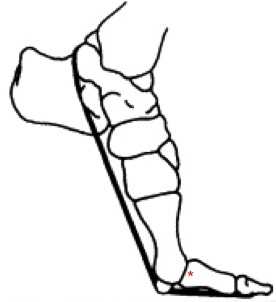
Now here’s that joint in the kadabba PPP4. The kadabba monograph has a nice midsagittal CT scan revealing this joint’s orientation, the angle of which I have measured using the free image analysis software ImageJ. kadabba‘s angle of ‘dorsal canting’ is 102.2 degrees. A mild fever.

Measuring the dorsal canting (the angle theta) of the AME-VP-1/71 proximal joint surface, using ImageJ.
This measurement is at the low end of the human range (averaging around 110 degrees for the 2nd, not 4th, digit), and above all but just a few apes analyzed by Griffin and Richmond (2010). Now, these authors looked at PPP2s, but PPP4s would be more appropriate for comparison with kadabba. LUCKY YOU – your students can collect these data, using CT scans from the KUPRI digital morphology museum. This collection has dozens of apes and monkeys (and even some other mammals), presumably none of which were habitually bipedal, and which should have relatively low angles of canting. (many of these specimens are from zoos, however, so their activity patterns and anatomies may not be the same as wild animals’; lookit the gorilla below) Your students can isolate and section proximal pedal phalanges as I have below, and measure the angle of canting with ImageJ. SCIENCE!

Easy image acquisition on the KUPRI database (this is a gorilla, with a pretty messed up fourth digit beyond the distal PPP). Have your students save the sectioned image as above, then measure the angle theta.
This activity is simple way for your students to set up a hypothesis, collect quality data and analyze them – essentially for free!
Some light weekend reading
Griffin and Richmond (2010). Joint orientation and function in great ape and human proximal pedal phalanges. American Journal of Physical Anthropology 141: 116-123.
Haile-Selassie (2001). Late Miocene hominids from the Middle Awash, Ethiopia. Nature 412: 178-181.
Haile-Selassie and WoldeGabriel, eds. (2009) Ardipithecus kadabba: Late Miocene Evidence from the Middle Awash, Ethiopia. Chapter 7.
Haile-Selassie et al. (2012). A new hominin foot from Ethiopia shows multiple Pliocene bipedal adaptations. Nature 483: 565-570.
Latimer and Lovejoy (1990). Metatarsophalangeal joints of Australopithecus afarensis. American Journal of Physical Anthropology 83: 13-23.
Lovejoy et al. (2009). Combining prehension and propulsion: The foot of Ardipithecus ramidus. Science 326: 72e1-72e8
It’s only Valentine’s Day, and already early 2014/late 2013 have provided several fascinating, high profile studies of ancient DNA (all been published in Nature). Forecasting this deluge, last year closed with the announcement of sequenced mtDNA from a ≥400,000 year old human fossil from Sima de los Huesos, Spain (Meyer et al., 2013). This is the oldest DNA obtained for any human fossil, and among the oldest of any animal.
Shortly thereafter, Prüfer and pals (2014) published the complete genome of a Neandertal from the infamous Denisova cave. This study revealed extensive inbreeding in Siberian Neandertals; the fossil individual’s high level of homozygosity is consistent with their parents being half-siblings. Furthermore, comparison of the genome of this inbred Neandertal with modern humans’ allowed researchers to identify many mutations that have become fixed (shared by all people) by natural selection since the divergence of our and Neandertals’ ancestors. Uncovering these human-specific variants can help us understand the genetic bases for many of humans’ remarkable traits.
In January, Olalde y coautores published a genomic analysis of a 7,000 hunter-gatherer from Spain. This ancient genome contained ancestral variants for genes relating to skin pigmentation (SLC45A2, SLC45A5, MC1R, TYR, and KILTG), meaning this Mesolithic European most probably had dark skin. This individual also had a derived variant of the HERC-OCA2 locus, associated with blue eye color in present day people. This suggests that the relatively novel phenotype of non-brown eyes may have increased in frequency more quickly than light skin color in ancient Europe. This guy also had many derived loci associated with immune function, indicating that the rise of agriculture is not solely responsible for the evolution of immune function in present day Europeans.
Around the same time, Sankararamen and team published an analysis of the distribution of Neandertal genes in living people. Whereas previous studies had already shown that Neandertals contributed ≤4% on average to the genomes of living people, this study examined where in modern people’s genomes this Neandertal ancestry tends to be located. One of the most interesting findings is that Neandertal genes are not uniformly or randomly distributed across the modern human genome. Rather, some regions appear to be especially devoid of Neandertal ancestry, implying natural selection acted strongly against Neandertal genes. These Neander-nude areas are preferentially found on the the X chromosome and in genes expressed in the testes, a finding consistent with reduced fertility in hybrid males. Although the genetic contribution of Neandertals to modern humans means that the two belonged to the same species, Sankararaman et al’s findings suggest the two groups were on their way to becoming different species.
Finally, this past week Rasmussen and rascals have published an analysis of a 12,000 year old human from the Anzick site in Montana, associated with the Clovis stone tool culture. I don’t know much about this time period save for what I learned in a class on North American archaeology taught by Dr. John Speth, back when I was a young, bright-eyed graduate student. One thing I recall from this class, when we were going over Clovis, was that this tool industry was found all over the United States at the beginning of the Holocene, but I was always disappointed by the dearth of bones complementing the copious lithics. Turns out, the DNA analyzed by Rasmussen et al. comes from the only known burial from this time period. This lone burial provides compelling genetic evidence that indigenous Americans have descended largely from a single ancestral population that separated into the North and South American populations prior to the Clovis period. This ancestral population was definitely not from Europe, as a minority of researchers have argued. Check out the SEAC Underground blog for more on the archaeology and ethics of the Anzick analyses.
So, paleogenomics is really crushing it right now. There have been many of recent advances in sampling and sequencing poorly-preserved ancient DNA, and as we’re seeing now, lots of ancient bones (and teeth) are bringing awesome new, genetic insights into recent human evolution. If this is how well we’re doing so early in 2014, you can bet that the rest of the year promises many more exciting discoveries.
I teach Tuesdays and Thursdays this year, leaving Fridays welcomely wide open for non-teaching related productivity. Today’s task is arguably the most exhilarating aspect of doing Science – inspecting raw data to make sure there are no major errors or problems in the dataset, so I can then analyze it and change the world. The excitement is truly hard to contain.
No, it’s not the funnest, but it’s an important part of doing Science. To make your life easier, you should inspect data daily as you collect them. This way, you can identify mistakes and make notes about outliers early on, so that you are not stupefied and stalemated by what you see when you sit down to begin analysis.

You (corgi) are getting ready to analyze and you find an anomalous observation (door stop) you didn’t notice when you were collecting data.
Today I’m looking at measurements I took from ape mandibles housed in an English museum last summer; I inspected data before I left the UK for KZ, so today should be a breeze. But no matter how meticulous you are in the field/museum, you still need to inspect your data before analyzing them, just to be safe. If you’re as disorganized as I am, there will be lots of programs each with lots of windows. Here’s a tip: plug into multiple monitors (or at least one big ass monitor), so you can easily espy all open windows and programs in prodigious panorama.

Using two monitors helps when checking data for errors and patterns. On my left screen I’m using R to visualize and examine the raw data open in Excel on the right screen. If something seems off on the left screen, I can quickly consult the original spreadsheet on the right.
Barely visible in the above screenshot, these are chimpanzee (red) and gorilla (black) mandible measurements plotted against a measure of body size, preliminarily described in this post from last August. I’m looking at whether any mandibular measurements track body size across the subadult growth period, in hopes that bodily growth can be studied in fossil species samples dominated by kid jaws. As you can (barely) see, some jaw measurements correlate with body size better than others, and sometimes the apes follow similar patterns but other times they don’t.
The data look good, so now I can go on to examine relationships between mandible and body size in more detail. Stay tuned for results!
Over the holiday break I was working at a cafe, and was shocked to find the upholstery besprinkled with bones. Looking at this seatback, can you tell what kinds of bones, and from whom, adorn this food establishment?
Of course there’s no one right answer, but what I saw were the undeveloped shafts of infant limbs. Infants?! Mildly morbid, mayhap, but one of the distinguishing features of juvenile limb bones compared with adults is that babies’ epiphyses (joint ends) are not fused to the shafts. Observe:
Each of the newborn bones pictured above is comprised of a shaft (diaphysis) that flares proximally and distally into a ‘metaphysis.’ In adults, the epiphyses are completely fused to the metaphyses, but in juveniles the epiphyses are separated from metaphyses by a growth plate made of cartilage. Different epiphyses tend to fuse at characteristic ages, and when fusion occurs bone growth ceases.
Functionally, this cartilage growth plate allows the bones to increase in length, as multiplying cartilage cells are replaced by bone cells. Because the epiphyses of different limbs fuse at different times, this means that limb proportions change subtly over the course of growth. Practically, this means that if an archaeologist (or forensic scientist or paleontologist) finds a limb shaft with unfused ends, he or she can estimate the age at which the individual may have died:

Standards for epiphyseal fusion. Same bones in same order as in previous figure (also from Scheuer and Black, 2000). “A” refers to the age (years) when the epiphysis firsts appears, and “F” to when it fuses to the shaft.
So if we assume the bones in the second figure are from the same person, we see a humerus, femur and tibia with completely unfused epiphyses. If we refer to our aging standards (third figure), we can see that the first epiphysis to fuse is the proximal humerus, between 2-6 years, and the next epiphyses to fuse are the distal humerus and femur head/proximal tibia between 12-14 years. So we could conclude that this poor kid was certainly younger than 12, years, if not even younger than 2 years. Again, having more of the skeleton (especially jaws with developing teeth) would help us make a more precise estimation.
Baby bones all over the place?! Shame on you, Panera.
GET THIS BOOK: Scheuer L and Black S. 2000. Juvenile Developmental Osteology. Academic Press.
A new year is upon us, our hair is a bit grayer and our telomeres a touch trimmer. Twenty effing fourteen.
It’s been a bit quiet here at Lawnchair, as I’ve been enjoying the holidays, but also writing a few things up for print. If I weren’t so old and wise, I’d make a New Year’s resolution to add to the blog more frequently. But I have a nascent career to attend to! So in the mean time, with the new year and semester, I’m adding two new courses to the Nazarbayev University bioanthro student blog that can hopefully keep you entertained & edumacated.
The first batch of student-written posts for the class “Bones, stones and genomes: Human Evolution” will go up on Monday. There will be a slight lull for a few weeks until this class, as well as “Monkey business: Primate behavior and ecology,” start posting in February. In addition to what’s already been posted by last year’s classes, the human evolution class will be adding posts focused on specific bones and fossils, while the primatology class will be adding article reviews/summaries.
So stay tuned to nazarbioanthro.blogspot.com in the coming months! (I should also have more fun new things to say here at Lawnchair, too)
If hell were around 400,000 years old. The people who salvaged ancient DNA from fossil Neandertals and “Denisovans” now present mitchondrial DNA (mtDNA) from a human-ish fossils from the Spanish site of Sima de los Huesos (SH; this translates as “pit of bones,” by the way, which is pretty badass). DNA-bearing Neandertal sites and Denisova cave date anywhere from around 30-100 kya, while Sima de los Huesos has been dated by various methods to 300-600 thousand years ago. So the newly announced mtDNA is the oldest human DNA ever recovered…
YET!
Now, we know what Neandertals look like, since they are perhaps the best known group of fossil humans. We don’t really know what Denisovans look like, as their unique DNA came from fossils that are anatomically ambiguous (a large molar and the end of a tiny fragment of the bone at the end of your pinky finger) – they could look like anyone. Even you! The SH fossils predate Neandertals by a few hundred thousand years, but their skulls look pretty similar; quite possibly the SH populations were ancestors of Neandertals, and you’d expect the DNA to be similar in the two groups.
So researchers were surprised to find this SH mtDNA to be more similar to Denisovan than to human or Neandertal mtDNAs. But this actually shouldn’t be that surprising, since we saw the same twist when Denisovan mt and nuclear DNA was sequenced – mtDNA first made it look like humans and Neandertals were more closely related, and the ancestors of Denisovans separated from the human+Neandertal lineage in the deep past. However, mtDNA essentially acts as a single genetic locus – a gene tree isn’t necessarily a species tree – and the more informative nuclear DNA later showed Neandertals and Denisovans to be more closely related to one another than either was to living humans (yet each of these ancient populations contributed some genes to some living people today). Denisovans held on to a very ancient mtDNA lineage, and apparently so did the people represented at Sima de los Huesos. And let’s not forget, we don’t know what Denisovans looked like – maybe they looked just like the older SH fossils.
Hopefully we’ll be able to get human nuclear DNA from Sima de los Huesos. When we do, I predict we’ll see the same kind of twist as with the Denisova DNA, with SH being more similar to Neandertals. But if I’m wrong, maybe we’ll be a step closer to knowing what the bones of the the mysterious “Denisovans” looked like…
Here’s that paper: Meyer et al. in press. A mitochondrial genome sequence of a hominin from Sima de los Huesos. Nature. doi:10.1038/nature12788
As was predicted long ago, and is becoming increasingly apparent, many anatomical differences between individuals are due not so much to the DNA coding for specific proteins (“genes”), but rather to the DNA that helps regulate when, where and how much these genes are expressed. A recent paper by Catia Attanasio and colleagues have identified thousands of these latter regions that appear to influence the development of facial shape, using a mélange of modern molecular, microscopic & morphometric methods. This is an exciting step toward understanding the genetic bases of facial variation within, and probably between, species.
Attanasio and colleagues identified “enhancers,” bits of DNA that enhance or increase the transcription of certain genes, relating to the embryonic development of the face. One interesting thing about these enhancers is that they aren’t usually found within the genes they enhance, but may be as far away as a few hundred thousand nucleotides. This is part of why these regulatory elements can be so hard to ascertain. What’s more, in the researchers’ own words, enhancers “often control the expression of their target genes in a modular fashion, where different enhancers activate the expression of the same gene in different cell types, anatomical regions, or at different developmental time points.” So in addition to the difficulty in finding enhancers, their varied ‘behavior’ makes it difficult to figure out exactly what each one does.
I won’t get into the methods they used to do this, but basically they were able to visualize when and where many of these enhancers were active in the developing face of mouse embryos. They also showed that tinkering with these enhancers had characteristic effects on bony facial shape in adults. The results are amazing:

Figure 5 from the paper. Blue/red indicate presence of a given enhancer. The white/blue images are actual mouse embryos, from younger (left) to older (right). Each green/red image is a 3D reconstruction of the blue/white embryo above, based on optical projection tomography.
Science has also made a very informative and visually stunning video to accompany the paper. Check it out. NOW.
So. Facial shape is the result of massively complex interactions between not just numerous genes, but also the coordination of thousands enhancers and other types of non-coding DNA regulating gene expression. Many other studies have tried to uncover the genetic bases of complex phenotypes (usually diseases) via genome wide association studies (GWAS), scanning genomes for shared genetic variants between individuals with similar phenotypes (I discussed this approach briefly Friday). In contrast to GWAS, what I really like about this study by Attanasio and colleagues is that they not only identify specific stretches of DNA as enhancers, but they also mapped their activity in developing embryos. Thus they could actually see how genetic variants contribute to phenotypes.
This is an important step toward understanding exactly how various genetic diseases affecting the face manifest. In addition, this and other studies uncovering the complex molecular interactions influencing facial shape could form the bases for computational models of development, to predict the genetic and developmental origins of facial evolution.
The paper: Attanasio C et al. 2013. Fine tuning of craniofacial morphology by distant-acting enhancers. Science 342: 1241006.
The topic this week in my Human Variation and Race class is intelligence. We’ve read about and discussed what intelligence is, how it is quantified, and the extent to which ‘intelligence,’ however defined, is biologically and/or environmentally determined. Intelligence (test score) has been shown to be heritable, meaning that a proportion of the variation in IQ test scores in a population can be explained by genetic variation. But that is not the same as saying that it is genetically determined. Similarly, complex traits such as intelligence, behaviors, and diseases almost never have a simple genetic basis – a common theme over at the Mermaid’s Tale, one that seems too rarely heeded. So you can imagine my surprise and delight at finding this news piece just published in Nature: “Root of maths genius sought: Entrepreneure’s ‘Project Einstein’ taps 400 top academics for their DNA.” Of course “roots” meant “genes.”
Apparently, bioinformatics entrepreneur and multimillionaire Jon Rothberg has set out to identify the genetic bases of peak mathletics, by analyzing the genomes of hundreds of mathematicians and physicists. Good luck, buddy! My initial reaction was to be appalled that an educated biologist these days could be such a flagrant biological determinist. What’s more, when approached about participating in the study, mathematician Curtis McMullen asked about the ethics of the project and its outcomes: “The uniform answer to my questions was that ‘we are not responsible for how the information is used after the study is completed.'” Ew. The project as briefly described reeked of some eugenics programme.
My prediction is that if this study takes off, Rothberg & buddies will be horribly disappointed. Assuming they are able to identify any genetic variants, these will probably only explain a small amount of variation in “maths genius.” Which itself is problematic, since there is probably not a single manifestation of math genius, and even if there were a single way to be a math genius, there may be several genetic pathways relating to the phenotype (not an uncommon finding of many genome-wide association studies). But hey, it seems to be Rothberg’s own money going into the study, so why not.
But then, if my prediction were to hold, this wouldn’t necessarily be a failure – it would point to an important role of society and learning environment in shaping individuals’ mathematic capability. And then maybe big money could begin to be diverted to more productive programs investigating and improving how people learn, rather than to large scale projects seeking simple answers when there isn’t necessarily any reason to expect them in the first place.