Osteology everywhere: Graffiti

January 20, 2015May 27, 2015 / zcofran / 1 Comment

Astana, the wedding-cake capital of Kazakhstan, is notably bereft of graffiti and street art, at least in my somewhat limited exposure to the city. The larval metropolis is all about commercial appearance, so I’d guess that aspiring street artists likely face much more than the Marge Simpson treatment for turning around to brag about their work.

Dire consequences await those who graffito tag public property.

Once, I did see a pretty badass street mural,

but it was in München, a mere 2,620 miles from Astana.

No, there is not much in the way of secretly donated street art here in Astana, and there’s generally little hope to see graffiti-grafted Osteology Everywhere. But this weekend, I noticed these four magical letters, quickly quietly scrawled on the side of my apartment building:

DAKA.

Two disconcerting thoughts immediately come to mind reading this. First, why the hell is “DAKA” written in Latin instead of Cyrillic script characteristic of the FSU? Second, what does “DAKA” mean out here? Nothing in Russian so far as I know, but Google Translate claims it could mean “Dakar” in Kazakh, which if true raises even more questions.

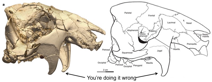
No, the safest assumption is that this tagger, my streetwise and marker-wielding dopplegänger, was referring to the ~1 million year old Homo erectus partial skull from Ethiopia, dubbed “Daka” after the Dakanihylo site of its discovery.

The Daka calvaria (Figure 2. of Asfaw et al., 2002). Counterclockwise from the top left: view from the back, view from the top (front is to the left), view from the left, a mosquito net, view from the bottom (front is at the top), viewed from the front.

BOU-VP-2/66, the Daka calvaria* (Figure 2. of Asfaw et al., 2002). Counterclockwise from the top left: view from the back, view from the top (front is to the left), view from the left, a mosquito net, view from the bottom (front is at the top), and view from the front. *Calvaria is the fancy word for ‘bony skull without a face.’

Daka isn’t the first hominin fossil to be embraced outside of anthropology. A few years ago I noticed the 4.4 million year old Ardipithecus ramidus skeleton strutting across the label of a Dogfish Head beer bottle:

GOODGRIEF, this was almost 5 years ago.

In downtown Tbilisi, Georgia I recently spotted a Dmanisi-based duo whose tech savvy belies the fact they’re based on 1.8 million year old fossils:

(Let’s not forget this one, from before they got smartphones)

We’ll have to do some serious fossil-finding here in Kazakhstan before they’ll let anyone put up something this awesome on the side of anything here in Astana. (Or wait…)

eFfing #FossilFriday: Subfossil lemurs

January 9, 2015January 1, 2016 / zcofran / 1 Comment

Hard to resist the headline, “Enormous underwater fossil graveyard found,” from the National Science Foundation. The NSF posts a video detailing the discovery of an underwater cave system containing “hundreds of potentially 1,000-year-old [lemur] skeletons…” in Madagascar. As a paleontologist, hearing about the discovery large numbers of ancient skeletons is musical, like hearing Love This Giant or the new T Swift for the first time.

Two lemur crania in an underwater cave on Madagascar. Photo from nbcnews.com.

It’s a pretty remarkable discovery – hundreds if not thousands of bones representing many complete skeletons of various extinct lemur species. And toward the end of the clip is a skull of a pretty badass looking big cat. The video shows piles of loose bones dredged up from the cave. These will reveal lots of information about the biology of these recently extinct animals, especially if researchers can keep associated bones together.

So what are these animals? Lemurs are one of the most primitive living types of primates – although they are relatively closely related to us humans, they retain many characteristics of ancestral mammals. I know it’s hard to believe this aye-aye here is more closely related to you than to rodents, but it is:

An aye-aye (Daubentonia madagascarensis) using its narrow and elongated middle finger to fish for for grubs inside a tree that it’s opened up with its teeth.

Lemurs are found only on the island of Madagascar, and over the past several millions of years they have diversified into the roughly 100 species inhabiting the island today. But even just a few thousand years ago, there were more kinds of lemurs. This includes Megaladapis, the large-bodied “koala lemur,” and Hadropithecus, whose skull bears a striking resemblance to the extinct hominin Australopithecus boisei. As Laurie Godfrey says in the video, “two thirds of the animals that lived there only a thousand years ago are gone.” Humans are probably largely responsible for the extinction of many Malagasy lemurs in both the past and especially the present.

Much of the ‘fossil’ record for lemurs is recent by fossil standards, and so most specimens haven’t become fully fossilized. As a result, lemur paleontology is besprinkled with the term “subfossil,” indicating bones that are really old and belong to extinct animals, but don’t fit the technical definition of fossils. The lemur subfossil record has taught us a lot about the evolutionary history, adaptations, and recently even genetics of this primitive group of primates, as well as about the ecological history of Madagascar. It will be very interesting to see what new insights will come from the recently discovered scores of underwater skeletons.

OH NO IT’S HADROPITHECUS

(Figure 3 from Ryan et al., 2008. Scale bar is 1 cm)

Another small Middle Pleistocene person

January 7, 2015January 1, 2016 / zcofran / 1 Comment

Last year I brought up the implications of the small female pelvis from Gona, Ethiopia for body size variation in Homo erectus (see previous post). This individual was much smaller than other Middle Pleistocene Homo fossils, indicating size variation comparable to highly sexually dimorphic gorillas and unlike recent human populations. Before this pelvis, most known Homo erectus fossils were fairly large (comparable to living people), with only a few hints of much smaller individuals (e.g., KNM-ER 427000, KNM-OL 45500). Now joining this petite party, this tiny troop, this little lot, this compact cadre, etc., is KNM-WT 51261, a 750,000 year old molar from Kenya (Maddux et al., in press).

Occlusal area for hominin first molars. The tooth is from Fig. 2 and the plot from Fig. 3 in the paper.

Occlusal area for first molars in the genus Homo. The tooth image is from Fig. 2 and the plot from Fig. 3 in Maddux et al. Lookit how tiny it is!

This ‘new’ specimen substantially increases the range of size variation among early African H. erectus molars, although the expanded range isn’t remarkable compared with later Homo samples such as from Zhoukoudian cave in China or Neandertals. What is different, though, is that most of the highly variable samples show a fairly continuous range of variation, while the WT 51261 molar is a considerable outlier from the rest of the African Middle Pleistocene sample (a lot like the situation with the Gona pelvis). So this tooth re-raises an important question: were smaller specimens like Gona and WT 51261 as rare in life as they are in the fossil record, or was such great size variation common in the Middle Pleistocene? How we reconstruct what kind of animal Homo erectus was differs depending on the answer to this question.

Driving nails into the 2014 Lawn Chair

December 30, 2014January 14, 2015 / zcofran / 1 Comment

It’s that time again, when we come to bury the year we’ve just defeated, only to celebrate the zombie birth of a new onslaught of days to clobber. In the spirit of auld lang syne, let’s recap the highlights of Lawn Chair in 2014.

Osteology was everywhere: although I am wont to see bones everywhere in everyday life, this year I only wrote about it four times. First there were the baby bones in cafe upholstery in my hometown of Kansas City, then the giant sheep bones in my new home of Astana. I discovered that animal bones littered the landscape of desert Mangystau, and then I spotted a vertebra hiding in a helmet at a conference in Italy. I also tweeted about a false femur head from a karaoke bar in Astana. You can’t escape. 2015 is sure to be more osseous.
eFfing Fossil Friday reboot: This old series focusing on fossils furtively restarted on a plane, when I uncovered the conspiracy that the Australopithecus africanus cranium Sts 71 was actually the Kryptonian codex. I later wrote about the Sima de los Huesos skulls, Neandertal poop, the origins of feathers on badass dinosaurs, the 45,000 year old Ust’-Ishim femur and its delicious DNA, and facial flanges in early mammals and nearly modern baboons. Fossils are the best, and 2015 is bound to be as fossiliferous as last year.Ancient DNA was boss: In addition to the earliest ‘modern’ human DNA from Ust’-Ishim, 2014 also witnessed a swath of studies early on attesting to the success of paleogenomics. We also got a first glimpse into epigenetics of ancient humans, and the potential importance this will have in uncovering how our DNA makes us human. Along these lines, for 2015, I’d be keen to see more work on miRNA and other aspects of gene regulation in ancient genomes.

R codes: I’ve posted R code for the analysis from my paper that came out this year, comparing mandibular growth in humans and Australopithecus robustus (I didn’t get to talk about that paper when it came out because I was in the middle of the Rising Star Workshop. Things to look forward to in 2015…). I’ll also be posting code for the analysis of brain growth in Homo erectus once that paper is published, and I have already posted code for creating the pretty pictures from the paper.

Body size variation in Homo erectus: A response to a response to a paper led me to reexamine sexual dimorphism in body size in our early ancestor – seems it was higher than has lately been appreciated, and there are many potential reasons for this. I presented the initial results of this investigation on the blog and at a conference, and am now writing this up for publication. This investigation is based on resampling statistics, nothing as new and flashy as in the growth studies. I will post code for these analyses on the R Codes page in due time.

Resampled ratios of dimorphism, calculated by dividing the average of six randomly selected male body masses by a randomly selected female mass. The blue star in each plot is the empirical ratio of average male mass/average female mass. For all species the average resampled ratio is almost identical to this empirical value. The red line marks the ratio of the six largest (male?) Homo erectus mass estimates divided by the estimated mass of the Gona (female?) pelvis. The Homo erectus male/female difference is rarely observed in chimps and humans, but is common in gorillas. Gorillas display high levels of sexual dimorphism, suggesting this may have been the case for Homo erectus as well.

Classroom lab activities: This year I added a lab components to my courses here at NU, and I posted up two of the lab activities I did in my classes this semester. Last spring, I got the idea for an activity in which students measure toe joint angles on digital images, to test whether Ardipithecus kadabba and other hominin toes can be distinguished from apes’. This semester, students in my human evo-devo class did this study, and generally found hominin toes to be more angled than apes’. Hypothesis tested. My Intro to Bio Anthro class tested whether their limb proportions fit expectations based on Allen’s Rule, and mystery ensued. My classes next term aren’t as conducive to lab activities, but if I come up with any good assignments I’ll be sure to post them.

Now that 2014 is laid to rest, here’s to a bright and successful zombied 2015! Жаңа Жылыңызбен!

2015 AAPA conference: More brain growth

December 13, 2014January 17, 2015 / zcofran / Leave a comment

The American Association of Physical Anthropologists is holding its annual meeting next year in St. Louis, in my home state of Missouri (I’m from Kansas City, which is by far the best city in the state, if not the entirety of the Midwest). I’ll be giving a talk comparing brain size growth in captive and wild chimpanzees, on Saturday 28 March in the Primate Life History session. Here’s a sneak peak:

Velocity curve for brain size from birth to 5 years in wild (green) and caprive (blue) chimpanzees. For the captive models, the dashed line is fit to the raw brain masses, and the solid line is fit to the estimated endocranial volumes.

Velocity curves for brain size growth from birth to 5 years in wild (green) and captive (blue) chimpanzees. The wild data are endocranial volumes, but the captive specimens are represented by brain masses. So the captive data are modeled for both the original masses (dashed) and estimated volumes (solid). Wild data are from Neubauer et al. 2011, captive data from Herndon et al., 1999.

Abstract: This study compares postnatal brain size change in two important chimpanzee samples: brain masses of captive apes at the Yerkes National Primate Research Center, and endocranial volumes (ECVs) of wild-collected individuals from the Taï Forest. Importantly, age at death is known for every individual, so these cross-sectional samples allow inferences of patterns and rates of brain growth in these populations. Previous studies have revealed differences in growth and health between wild and captive animals, but such habitat effects have yet to be investigated for brain growth. It has also been hypothesized that brain mass and endocranial volume follow different growth curves. To address these issues, I compare the Yerkes brain mass data (n=70) with the Taï ECVs (n=30), modeling both size and velocity change over time with polynomial regression. Yerkes masses overlap with Taï volumes at all ages, though values for the former tend to be slightly elevated over the latter. Velocity curves indicate that growth decelerates more rapidly for mass than ECV. Both velocity curves come to encompass zero between three and four years of age, with Yerkes mass slightly preceding Taï ECV. Thus, Yerkes brain masses and Taï ECVs show a very similar pattern of size change, but there are minor differences indicating at least a small effect of differences in habitat, unit of measurement, or a combination of both. The overall similarity between datasets, however, points to the canalization of brain growth in Pan troglodytes.

Kazakhstan’s killer cats

December 6, 2014 / zcofran / 1 Comment

I’m reading up on previous paleontological research that’s taken place here in Kazakhstan, planning for future work. There aren’t any human fossils known from here (at least, none to my knowledge). But, I did stumble upon this badass, sabre-toothed cat from the Late Miocene (over 5 million years ago):

From Sotnikova, 1992. Original caption: Fig. 2. Machairodus kurteni, Kalmakpai (PIN-2433/287), skull, ventral and lateral view.

From Sotnikova, 1992 (mandible not shown). Original caption: Fig. 2. Machairodus kurteni, Kalmakpai (PIN-2433/287), skull, ventral and lateral view.

The skull was described by MV Sotnikova in 1992, and comes from a site called Kalmakpai in the Zaysan Basin in East Kazakhstan. For perspective, Sotnikova says the skull is about the same size as an adult African lion. This is much larger than the wildlife I’ve seen lately in snow-soaked Astana (I trailed a large white rabbit in Presidential Park by the river on my run today. Not as badass).

This is a reminder that the Big Cats once had a much larger geographical distribution than they do today. The skull above belongs to the genus Machairodus, which is also known from Africa, Europe and North America. Machairodus is closely related to Homotherium, another large, geographically dispersed genus of sabre-toothed cat from the Pliocene (including at Dmanisi).

Of course, extinction isn’t exclusive to the deep past: the Caspian Tiger used to roam parts of southern Kazakhstan and other areas of Central Asia, going extinct only in the past few decades.

Results of the toe-tally easy lab activity

December 3, 2014 / zcofran / 4 Comments

Alternate title: Dorsal canting in primate PPP4s

Earlier this year I suggested a classroom activity in which students can scrutinize the evidence used to argue that the >5 million year old (mya) Ardipithecus kadabba was bipedal. To recap: Ar. kadabba is represented by some teeth, a broken lower jaw, and some fragmentary postcrania. The main piece of evidence that it is a human ancestor and not just any old ape is from a single toe bone, and the orientation of its proximal joint. In Ar. kadabba and animals that hyperdorxiflex their toes (i.e., humans and other bipeds when walking), this joint faces upward, whereas it points backward or even downward in apes. This “dorsal canting” of the proximal toe joint has also been used as evidence that the 4.4 mya Ardipithecus ramidus and 3.5 mya owner of the mystery foot from Burtele are bipedal hominins. A question remains, though – does this anatomy really distinguish locomotor groups such as bipeds from quadrupeds?

Use ImageJ to measure the canting angle between the proximal joint and plantar surface. Proximal to the right, distal to the left.

STUDENT SCIENTISTS TO THE RESCUE! Use ImageJ to measure the canting angle between the proximal joint and plantar surface, as I’ve done on this Japanese macaque monkey (they are not bipedal). Proximal to the right, distal to the left Note I changed the measured angle from the March post.

I sicked my students in Ant 364 (Human Evolutionary Developmental Biology) here at NU on this task. I had students look at only 11 modern primates from the awesome KUPRI database. Most groups are only represented by 1 (Homo sapiens, Hylobates lar and Macaca fuscata) or two (Pongo species and Gorilla gorilla) specimens, all adults. For chimpanzees (Pan troglodytes) there is one infant and four adults. The database has more individuals, and it would be better to include more specimens to get better ideas of species’ ranges of variation, but this is a good training sample for a class assignment. The fossil group includes one Ardipithecus ramidus, one Ar. kadabba, one Australopithecus afarensis, and the PPP4 of the mystery foot from Burtele. The human and all fossils except Ar. kadabba are based off of lateral photographs and not CT scans like for the living primates, meaning there may be some error in their measurements, but we’ll assume for the assignment this is not a problem. Here are their results:

Dorsal canting angle of the fourth proximal pedal phalanx in primates. The lower the angle, the more dorsally canted the proximal joint surface. The “Fossil” group includes specimens attributed to Ardipithecus, Australopithecus and something unknown.

Great apes have fairly high angles, meaning generally not dorsally canted proximal joint surfaces. The two gorillas fall right in the adult chimpanzee (adult) range of variation, while chimp infant and orangutans have much higher angles (≥90º means they’re actually angled downward or plantarly). The gibbon (Hylobates) is slightly lower than the chimpanzee range. The macaque has an even more dorsally canted joint, and the human even more so. The fossils, except the measurement for Ar. ramidus (see note above), have lower angles than living apes, but higher than the human and the monkey. If dorsal canting really is really a bony adaptation to forces experienced during life, then the fossil angles suggest these animals’ toes were dorsiflexed more so than living great apes (but not as much as the single monkey and human).

This lab helps students become familiar with CT data, the fossil record, taking measurements (students also measure maximum length of the toe bones and look at the relationship between length and canting), analyzing data, and hypothesis testing. You can also have fun exploring inter-observer error by comparing students’ measurements.

Here’s the full lab handout if you want to use or modify it for your own class: Lab 5-Toe instructions and report

Lessons from limb lab (activity)

November 16, 2014 / zcofran / 1 Comment

This semester I have added a lab component to my Introduction to Biological Anthropology class. Lab activities and assignments provide students with opportunities to gather data, to think about them in the context of various theories, and to learn about how to analyze them. This past week’s lab looked at limb proportions within our classroom, in the context of “Allen’s rule” – in colder climates, animals tend to have relatively shorter distal limbs (radius+ulna and tibia+fibula). Allen’s rule, along with “Bergmann’s rule,” describe ecogeographic variation in humans and other animals: body size (i.e., mass) and shape (i.e., limb proportions) tend to vary with climate, such that populations living in colder environments tend to have less surface area relative to body mass, as an adapation to retain body heat.

A simple and effective way to quantify the relative lengths of limbs is through ratios: in this case we examined the crural and brachial indices. Here I’ve plotted average human indices against latitude as reported in a recent paper by Helen Kurki and colleagues (2008):

Left: Crural index (tibia length/femur length) related to latitude, as a proxy for climate. Right: Brachial index (radius length/humerus length) plotted against latitude. Data from Kurki et al. (2008). Black=female, red=male. Dashed lines are regression slopes for each sex, and solid lines indicate the 95% confidence limits of the regression lines.

Human limb proportions related to latitude, as a proxy for climate. Left: Crural index (tibia length/femur length). Right: Brachial index (radius length/humerus length). Higher indices mean relatively longer tibia or radius. Data from Kurki et al. (2008). Black=female, red=male. Dashed lines are least squares regression lines for each sex, and solid lines indicate the 95% confidence limits of the regression lines. How well will our class’s data fit these models?…

These plots are consistent with Allen’s rule – the distal limb segments become relatively shorter with increasing latitude. In lab, we test whether our limb proportions reflect this presumably ecogeographic pattern. Here in Astana we are at 51ºN latitude, so these regressions predict that our class should have crural indices between 0.82-0.84, and brachial indices between 0.72-0.79. How well does our class fit these model’s predictions?

…Pretty terribly. Plots are same as above, except with our class’s data added at 51º N latitude (vertical lines). In each, the vertical lines span the class’s 95% range (black=females, red=males), with the dots marking each sex’s average. Kazakhstan is huge, and students could have grown up in latitudes from 42º-55º N, but even assuming students had all come from Shymkent their distal limbs still appear much longer than expected.

These plots show that students in the class have longer distal limbs than expected – both for our latitude, and for humans generally. The poor fit of my students’ limb proportions probably doesn’t mean they’re bad humans. Instead, we probably deviate because we compared apples to oranges: the Kurki data were dry long bones measured on an osteometric board, whereas I had my students do their best to palpate and measure the maximum lengths of their own bones beneath layers of fat, muscle, skin, and clothing. Our high indices probably reflect the underestimation of humerus and femur lengths, whose most proximal points that can be palapated (greater tubercle and trochanter, respectively) lie a bit lower than the respective heads, which would have been included in the Kurki measurements.

It was interesting to review these plots with students. Even though they’re fairly new at reading graphs like these, there was an audible gasp and bewildered muttering when their own data went up on the board. I myself was surprised at these results, but I’m happy with how the exercise went. This particular ‘study’ helps students learn about ecogeography, adaptation and human variation, as well as the importance of homology and comparing like with like.

eFfing Fossil Friday: Funky facial flanges #FFF

November 7, 2014April 29, 2016 / zcofran / 3 Comments

David Krause and colleagues announced in this week’s Nature the discovery of a new species of extinct mammal, Vintana sertichi, that lived in what is now Madagascar between 66-72 million years ago. The species is based on a very well-preserved cranium of an early gondwanatherian (if you want to impress your friends this weekend, gratuitously use the word “gondwanatherian”). I don’t know much about early mammals like this, but it sounds like it was a weird creature (see the Stony Brook press release). Just looking at it’s face there’s something that sticks out as strange:

Ventana sertichi cranium (Reich et al. 2014, Figure 1a). Left is a 3D CT reconstruction, right is a line drawing highlighting all the individual bones (so many cranial bones). The view is from the right side, so the nose is on the right, the eye is the big hollow in the middle, and the back of the skull is on the left. The jugal flanges are the downward projections.

Vintana sertichi cranium (Reich et al. 2014, Figure 1a). On the left is a 3D CT reconstruction, and on the right is a line drawing highlighting all the individual bones (so many cranial bones). The view is from the right side, so the nose is to the right, the eye socket is the shadowy hollow in the middle, and the back of the skull is on the left. The jugal flanges are the downward projections.

Jutting downward from the sides of the jaw are ‘jugal flanges,’ projections of bone on the homologs of human cheeks. Projections of like these usually serve as muscle attachment sites, and the size of the projection generally reflects the size of the muscle. These facial flanges anchor the masseter muscle, a major chewing muscle that helps close the jaw. The size of this flange in Vintana suggests its chomp packed a punch. A debilitating bite. A face not even a mother could love (so now they’re extinct).

Vintana‘s bony tear-catchers caught my eye because most primates I’ve seen have, you know, less heinous faces. Scouring the internet, big jugal flanges are a fairly rare sight, but can apparently be found in glyptodonts (giant, armadillo-like mammals that lived tens of thousands of years ago) and various sloths. The closest thing I’ve seen to this gross bony flange in Primates are on the zygomatic bones of some extinct, baboon-like animals, such as Dinopithecus ingens:

Fragmentary skull, viewed from the top, of Papio (a.k.a. Dinopithecus) ingens, from Swartkrans, South Africa. Photo credit: CalPhotos.

Fragmentary skull, viewed from the top, of Papio (a.k.a. Dinopithecus) ingens, from Swartkrans, South Africa. As a punishment for its zygomatic excess, its face was confiscated. Photo credit: CalPhotos.

and Theropithecus brumpti

Theropithecus brumpti from the Omo basin. Photo credit: CalPhotos.

Theropithecus brumpti from the Omo Basin, Ethiopia. Photo credit: CalPhotos.

So some primates dabbled in jugal flangery like Vintana, but Natural Selection was having none of it. Anyway, Vintana overcame this craniofacial adversity with characteristic Mesozoic moxie, and is an important piece in the puzzle of mammal evolution. It will be interesting to see what other mammalian surprises the Mesozoic has in store for paleontologists.

Can ‘ape-like’ actually be ‘human-like’?

October 29, 2014March 9, 2026 / zcofran / Leave a comment

I’m reading up on life history in Homo erectus for a few projects I’m working on, and something’s just caught my eye. A 2012 issue of Current Anthropology presents a series of papers from the 2011 symposium, “Human Biology and the Origins of Homo.” This issue is full of great stuff, and to top it all off, it can be accessed online for free! (here’s the JSTOR link)

Gary Schwartz has a paper here recounting what is known (or as he stresses, what is still largely unknown) about growth and life history in early Homo. Dental evidence accumulated over the past 30 years has pointed to a rapid (ape-like) life cycle for fossil hominins, in comparison with a slow, long and drawn out human pattern. But much of the evidence against a human-like pattern is somewhat indirect. For instance, Holly Smith (1991) has shown that there’s a pretty tight relationship between brain size and age at first molar (M1) eruption in Primates:

Fig. 1 from Schwartz (2012). “Bivariate plot of ln M1 emergence age in months (y) versus ln cranial capacity in cubic centimeters (x) for a sample of anthropoids.” The hominins and humans are the open shapes, to which I’ve visually fitted the red line.

It’s a very high correlation (r=0.98). This means that armed with simply an animal’s brain size (“cranial capacity” in the graph), which is fairly easy to estimate given complete enough fossils, one can estimate with a bit of confidence its likely age range for M1 emergence. With brain sizes between apes’ and ours, fossil hominins can be estimated to have erupted their M1s at younger ages than us. Many subsequent studies of tooth formation, based on the microscopic remnants of tooth development, have supported these inferences. So presumably, faster, ape-like dental development could be extrapolated to mean ape-like body growth rates and other aspects of life history as well.

But although this is a tight relationship, there are deviations. As Schwartz notes in the article, and others have noted before, high correlations found when examining large interspecific groups (e.g., primates as a whole) often break down when the focus is on smaller groups of more closely related species (e.g., just apes). Based on the relationship figured above, humans are expected to erupt M1 around 7 years of age, but nearly all humans erupt M1 closer to 6 years (hence the open diamond for humans is below the regression line). What hominins appear to share in common with humans is a younger age at M1 eruption than expected for primates of their brain sizes (the red line I’ve added to the figure).

Hominins’ faster dental development and eruption may be ape-like in absolute terms, but eruption ages may be human-like when their brain size is taken to account. As with many life history variables, the significance of this similarity (if anything) is difficult to ascertain.

Lawnchair Anthropology

Biological anthropology, paleontology, evolution, and development, by Dr. Zachary Cofran

Author: zcofran