The site’s been quiet in 2017, with little time to blog on top of my regular professional responsibilities, and of course watching the fascist smoke rising from the garbage fire of our 45th presidential administration with horrified disbelief. At work, my two new classes are keeping me plenty busy, and their content is quite distinct – one is on the archaeological record of Central Asia, the other centers around Homo naledi to teach about fossils. But by complete accident, examples of scientific racism came up in the readings for each course last week.

Scientific racism refers to using data or evidence from the biological and social sciences to support racist arguments, that one racial group is better or worse than another group; the groups of course, are culturally determined rather than empirically discrete biological entities. This evidence is often cherry-picked, misinterpreted, and/or outright weak. Nicolas’ Wade’s 2014 A Troublesome Inheritance is a recent example of such a work. The book’s racial claims amount to nothing more than handwaving, and so egregious is the misrepresentation of genetic evidence that nearly 150 of the world’s top geneticists signed a letter to the editor rebuking Wade for “misappropriation of research from our field to support arguments about differences among human societies.” Wade’s book has no place in scientific discourse, but then almost anyone can write a book as long as a publisher thinks it will sell.

In addition to the outright misrepresentation of scientific evidence to support racist arguments, another manifestation of scientific racism is the influence of cultural biases in the interpretation of empirical observations. This may be less malicious than the first example, but is equally dangerous as it more tacitly supports systemic and pervasive racism. And this brings us to my classes’ recent readings.

First was a reference to the “Movius Line” in a review of the Paleolithic record of Central Asia (Vishnyatsky 1999) for my prehistory class. Back in the 1940s Hallum Movius, archaeologist and amazing-name-haver, noticed a distinct geographic pattern in the distribution of early stone tool technology across the Old World: “hand-axes” could be found at sites across Africa and western Eurasia, while they were largely absent from East Asian sites, which were dominated by more basic stone tools.

Movius’ illustration of the distribution of Early Paleolithic technologies. From Fig. 1 in Dennell (2015).

Robin Dennell (2016) provides a nice review of how Movius’ personal, culturally influenced perception of China colored his interpretation of this pattern. Movius read this archaeological evidence to mean that early East Asian humans were unable to create the more advanced technology of the west, a biological and cognitive deficiency resulting from cultural separation: “East Asia gives the impression of having acted (just as historical China and in sharp contrast with the Mediterranean world) as an isolated and self-sufficient area, closed to any major human migratory wave” (Movius 1941: 86, cited in Dennell 2015). Racial and cultural stereotypes about East Asia directly translated to his interpretation of an archaeological pattern.

This type of old school scientific racism also arose in a review of endocasts (Falk, 2014) for my Homo naledi class. Endocasts are negative impressions or casts of a space or cavity, and comprise the only direct evidence of what extinct animals’ brains looked like. So to see how the structure of the brain has changed over the course of human evolution, scientists can search for the impressions of important brain structures in fossil human endocasts. Falk (2014) reviews one of the most famous of these structures – the “lunate sulcus” – which was used as evidence for reorganization of the hominin brain for nearly 100 years. In the early 20th century, anatomist and anthropologist GE Smith (not GE Smith from the Saturday Night Live Band)  thought he’d identified the human homologue of a groove that in apes separates the parietal lobe from the visual cortex. In humans, however, this groove was positioned more toward the back of the brain, which Smith interpreted as an expansion of an area relating to advanced cognition.

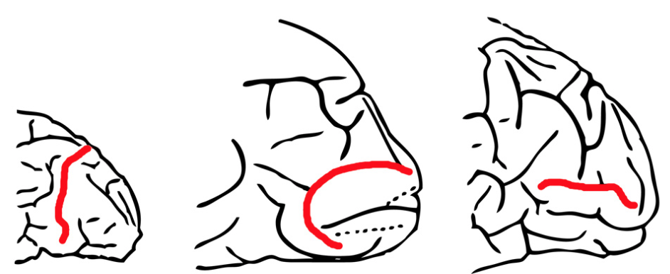
The back of the brain, viewed from the left, of a chimpanzee (left) and two humans, the red line illustrating the Affenspalte or lunate sulcus (Fig. 1 from Falk 2014, which was modified from Smith 1903). The middle one also might be a grumpy fish.

It turns out that the lunate sulcus does not actually exist in humans, as the grooves identified as such are not structurally or functionally the same as the lunate sulcus in apes (Allen et al., 2006). Nevertheless, given what Smith thought the lunate sulcus was, it’s tragic to read his interpretations of human variation: “resemblance to the Simian [ape] pattern… is not quite so obvious…. in European types of brain….” (Smith 1904: 437, quoted in Falk 2014). The human condition for this trait was for it to be located in the back, reflecting an expansion of the cognitive area in front of it, and this pattern was less pronounced, according to Smith, in non-European people’s brains. This interpretation reflects two traditions at the time: 1) to refer to racial ‘types,’ ignoring variation within and overlap between groups, as well as 2) the prevailing wisdom that Europeans were more intelligent or advanced than other geographical groups.

Anecdotes such as these may seem like mere scientific and historical curios, but they should serve as important reminders both that science can be accidentally guided by cultural values, or intentionally used for malevolent ends. Misconceptions and errors of the past shouldn’t be erased, but rather touted so that we don’t repeat mistakes that can have major consequences in our not-so-post-racial society.

References

Allen JS, Bruss J, & Damasio H (2006). Looking for the lunate sulcus: a magnetic resonance imaging study in modern humans. The anatomical record. Part A, Discoveries in molecular, cellular, and evolutionary biology, 288 (8), 867-76 PMID: 16835937

Dennell, R. (2016). Life without the Movius Line: The structure of the East and Southeast Asian Early Palaeolithic Quaternary International, 400, 14-22 DOI: 10.1016/j.quaint.2015.09.001

Falk D (2014). Interpreting sulci on hominin endocasts: old hypotheses and new findings. Frontiers in human neuroscience, 8 PMID: 24822043

Vishnyatsky L (1999). The Paleolithic of Central Asia. Journal of World Prehistory, 13, 69-122.