Update: Brain growth in Homo erectus, and the age of the Mojokerto fossil

The Mojokerto calvaria. You’re looking at the left side of the
 skull: the face would be to the left. Check it out in 3D here.

A few months ago I posted an abridged version of the presentation I gave at this year’s meetings of the American Association of Physical Anthropologists, about brain growth in Homo erectus. This study, co-authored with Jeremy DeSilva, adopts a novel approach (see “Methods” in that earlier post) to analyze the Mojokerto fossil (right). The specimen is the only H. erectus non-adult complete enough to get a decent estimate of brain size (or rather, the overall volume of the brain case) – probably 630 to 660 cubic centimeters (Coqueugniot et al. 2004; Balzeau et al., 2004). So to study brain growth in the extinct species, we just have to connect a range of estimated brain sizes at birth (around 290 cubic centimeters, based on predictive equations by DeSilva and Lesnik, 2008) to that of Mojokerto. But, the speed of brain growth implied by this comparison depends on how old poor Mojokerto was when s/he died.

Most recently, Hélen Coqueugniot and colleagues (2004) used CT scans of the fossil to examine the fusion of its various bones, to suggest the poor kid died between six months to 1.5 years, if not even younger. Antoine Balzeau and team (2005) also studied scans of the fossil, and their analysis of its virtual endocast presented conflicting age estimates, but they argued the poor kid was probably no older than 4 years. Earlier studies had suggested the kid was up to 8 years. Now, for my previous post/conference presentation, we assumed the Coqueugniot estimate was correct – but what if we consider a full range of ages for Mojokerto, from 0.03-6.00 years?

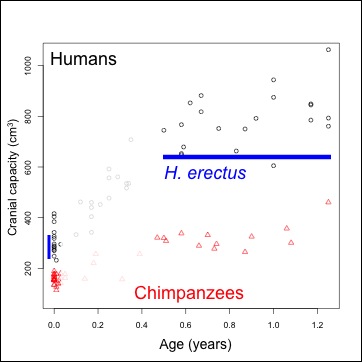
Brain size, relative to newborns’ values, at different ages in humans (black circles) and chimpanzees (red triangles). Homo erectus median and mean are the thick solid and dashed blue lines, respectively, and the 90% and 95% confidence intervals are indicated by the thinner, dotted blue lines. Data are the same as in the previous post.

The plot above depicts brain size relative to newborns: each circle (humans) and triangle (chimpanzees) represents the proportional size difference between a newborn (less than 1 week) and an older individual, up to 6 years. Obviously, relative brain size gets bigger in humans and chimpanzees over time. Interestingly, even though humans and chimps have very different brain sizes, the proportional brain size changes overlap a lot between species, especially at younger ages. Ah, the joys of cross-sectional samples.

But what’s especially interesting here are the blue lines on the graph, indicating estimates of proportional size change in Homo erectus, assuming Mojokerto’s skull could hold 630 cc of delicious brain matter, and that the species’ skulls at birth could hold about 290 cc, give or take several cc. The thick solid and dashed lines just above 2 on the y-axis are the mean and median of our estimates – Mojokerto’s brain averages around 2.2 times larger than predicted newborns. Such a proportion is most likely to be found in humans between 6 months to a year of age, and in chimpanzees between around 6 months and 2 years. The confidence intervals, the highest and lowest bounds of our estimates for Homo erectus proportional size change, are the thinner dashed lines on the graph. They help us constrain our estimates, and further suggest that the proportional difference found for H. erectus is most likely to be found in either chimpanzees or humans around 1 year of age – just like Coqueugniot and colleagues predicted!!!

Thus, independent evidence – brain size of Mojokerto and estimated brain size at birth in Homo erectus – corroborates a previously estimated age at death for the Mojokerto fossil, the poor little Homo erectus baby. This further supports our estimates of brain growth rates in this species, as described in the previous post.

ResearchBlogging.orgSo to summarize, fairly scant fossil evidence compared with larger extant species samples using randomization statistics, argue for high, human-like infant brain growth rates in Homo erectus by around 1 million years ago. Our ancestors were badasses.

Remember, if you want the R code I wrote to do this study, just lemme know!

Those references
Balzeau A, Grimaud-Hervé D, & Jacob T (2005). Internal cranial features of the Mojokerto child fossil (East Java, Indonesia). Journal of human evolution, 48 (6), 535-53 PMID: 15927659

Coqueugniot H, Hublin JJ, Veillon F, Houët F, & Jacob T (2004). Early brain growth in Homo erectus and implications for cognitive ability. Nature, 431 (7006), 299-302 PMID: 15372030

DeSilva JM, & Lesnik JJ (2008). Brain size at birth throughout human evolution: a new method for estimating neonatal brain size in hominins. Journal of human evolution, 55 (6), 1064-74 PMID: 18789811

We like turtles (‘s genomes)

June 2013, Volume 45 No 6 pp 579-714

Jonathan the zombie isn’t the only one who likes turtles. These heroes-in-a-half-shell adorn the cover of the current Nature Genetics, as two species of turtle have just joined the Genome Club (Wang et al. 2013; paper’s free!).

This definitely not one of those genome sequencing studies alluded to recently by John Hawks, that’s “too boring for journals.” Wang and colleagues didn’t just sequence the genomes of soft-shell and green sea turtles ‘just cuz.’ Rather, they use these copious data to address several questions, most interesting of which relate to embryonic development.

First, analysis of gene expression during embryonic development supports what the authors refer to as a “nested hourglass model” of development and gene expression. The hourglass shape serves as analogy for variation across related species over developmental time: there is great variation (in both morphology and gene expression) in the earliest stages of development, then species are more similar at a given developmental stage (the “phylotypic period”), and thereafter variation increases again. This phylotypic period (which I don’t believe is unanimously agreed upon) is arguably the most conserved developmental stage in evolution – all vertebrates, for example, simply must pass through this stage to become good vertebrates. Plus, several studies have found that evolutionarily younger genes tend to be expressed before and after this amorphous phylotypic stage, while more ancient genes are expressed during this time. As the authors state

“According to the recently supported developmental hourglass model … the changes underlying major adult morphological evolution occurred primarily in the developmental stages after the period … that serves as the basic vertebrate body plan.”

So the turtle data generally support this model. However they mention a nested hourglass, because they found evidence of an additional bottleneck, a second hourglass, of conserved gene expression when comparing turtles with their close relative the chicken. In other words, “the most conserved developmental stage changes depending on distantly related species are that are being compared.” So since turtles and chickens are more closely related to one another than to many other vertebrates, they might share another conserved developmental stage. Incidentally, both also make for good soup.

Wang and colleagues also looked for genes relating to some of the unique aspects of turtle anatomy, examining what parts of the genome seem to get kicked up after the phylotypic period. It doesn’t take a trained eye to see that these animals are kinda weird in that their bodies are encased in a flagrant shell, with a carapace on top and plastron on the bottom. Now it turns out this carapace is actually formed from what should, in most other vertebrates, become vertebrae and ribs. So by studying the earliest development of these structures, Wang and colleagues could examine the molecular bases of this carapacial deviation.

Fig. 5 from Wang et al., showing Wnt protein expression in turtle embryos. In a), only Wnt5a is expressed in the ‘carapacial ridge’ during its earliest development. Fig c) is a cross-section indicated in b) showing this expression. NT=neural tube, NC=  notochord. The scale bar is 0.5 mm. Tiny!
The authors were able to identify over 200 miRNAs, and implicate the signalling protein Wnt5a, in the development of the “carapacial ridge” (see the arrows in fig. c above), the embryonic precursors to the carapace. Interestingly, Wnt5a is involved in the development of limb buds (e.g, those big purple circles in the red square in a) above). The precise role of Wnt5a and the miRNAs in turtle shell development has yet to be determined, so this study really sets the stage for future investigations.
ResearchBlogging.orgSo there you have it, a pretty cool paper combining genomics with developmental biology, among other things. And so to close, for your bemusement, here’s a video I shot last week at the awesome Kansas City Zoo, of a turtle attempting to make embryos like in the figure above (sorry for the poor quality). Hang in there, little buddy!
They like tuhtles!
Wang Z, Pascual-Anaya J, Zadissa A, Li W, Niimura Y, Huang Z, Li C, White S, Xiong Z, Fang D, Wang B, Ming Y, Chen Y, Zheng Y, Kuraku S, Pignatelli M, Herrero J, Beal K, Nozawa M, Li Q, Wang J, Zhang H, Yu L, Shigenobu S, Wang J, Liu J, Flicek P, Searle S, Wang J, Kuratani S, Yin Y, Aken B, Zhang G, & Irie N (2013). The draft genomes of soft-shell turtle and green sea turtle yield insights into the development and evolution of the turtle-specific body plan. Nature genetics, 45 (6), 701-6 PMID: 23624526

Kazakhstan Paleolithic fieldwork: Valikhanova

Last week, I left my home in Astana for southern Kazakhstan, to rendezvous with researchers based in Kazakhstan, the United States and Germany. This is the beginning of a collaborative effort to understand the underappreciated importance of Kazakhstan in hominin evolution.

Post-fieldwork meal. From foreground clockwise: Zhaken Taimagambetov (1), Tyler (2), Saya (1), Jason (2), Adam (3), Radu (4), Mica (2), Kat (5), Katie (2), and Rinato (1). Not pictured: Me (6) and Jean-Marc (1). Numbers indicate school affiliations, at the end of the post.

We just returned from a brief stint of soil sampling at, and site surveying around, the Paleolithic site of Valikhanova, near the town of Zhanatas. This site was excavated decades ago, and has yielded a number of stone tools interpreted as transitional between Middle and Upper Paleolithic industries. This is a fascinating period for ‘modern’ human origins, but unfortunately the site has not yielded any human fossils to the best of my knowledge.

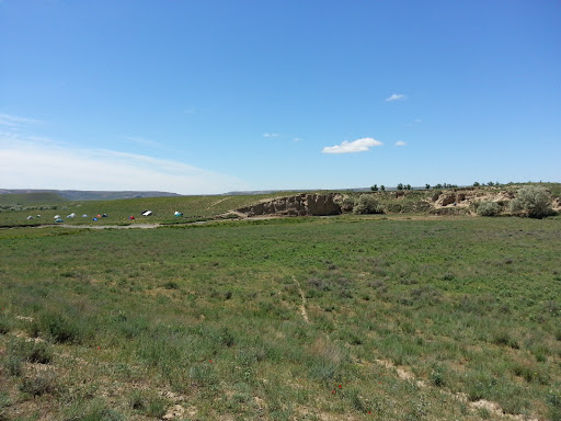
Valikhanova. The excavation site is the layered earth exposure on the right, our camp site on the left.

But there are other important questions that can be asked about the nature of the site and its inhabitants. First, the geological layers (“strata”) of the site have not been reliably dated, so soil samples were collected to be analyzed by a dating technique called optically stimulated luminescence (this is the work of Dr. Kat Fitzsimmons). Second, aspects of climate and ecology can be inferred from soil chemistry, which is the focus of team members from Colorado State University. Combining this information, we can begin to understand when and why humans (Neandertal and/or more ‘modern’ looking) inhabited the area – e.g., was it only between major glacial periods, how much time does the site span, etc?

And it’s a pretty amazing area. The site is nestled in a depression, creating an ecosystem somewhat protected from harsh winds and temperatures blowing around surrounding the mountains. That said, the night we arrived we were welcomed by extremely high-speed winds and heavy rains. My tent was the only casualty of the storm, forcing me to flee to the comforting confines of our sturdy truck and cups of vodka. The storm was short lived, and soon the sky opened up to a panoramic harlequin sunset.

Palette after the storm. Left to right covers from West to East. The excavation and North are at the center.

Also there was a rainbow.

My main activity here was survey, the search for other places that could potentially yield fossil and additional cultural materials. Survey basically involves a fairly targeted scouring of a landscape, searching for specific features. Our survey took us over and across gorgeous landscapes. We found a number of possible fossil/artifact accumulations and possible caves/rock shelters for future investigation, but no human fossils turned up (this was not terribly surprising, as human fossils are quite rare).

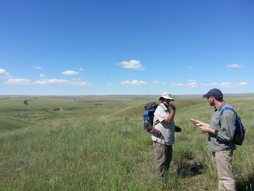
Atop one big hill, Drs. Jason LaBelle and Adam Van Arsdale discuss one of many stone tools we found littering the area around Valikhanova.

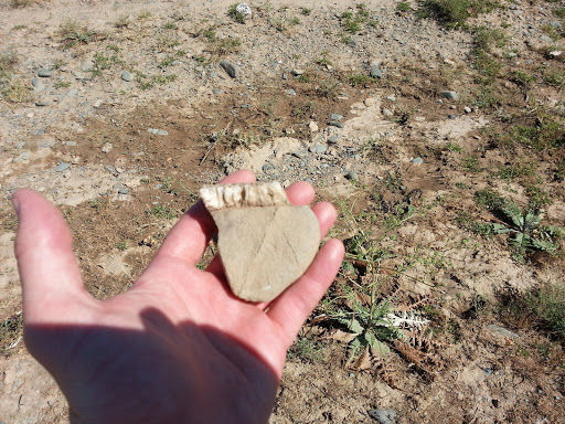
One neat surprise did come when scanning the ground above a rocky outcrop over a filled-in cave. At first glance, I seem to be holding some kind of a jaw bone fragmentwith two teeth. Close inspection shows this just to be a rock with a coincidentally-molar-like calcification. Bummer. However, we were able to trick one expert into thinking for a minute that we found some kind of pig or other mammal fossil.

Fossil bovid, equid or suid? Meganthropus?! Just a rock? Osteology students & paleontologists, beware faux-ssils…

We’re briefly back in Almaty to recharge, and on Tuesday we’ll head out to explore Charyn Canyon for a few days. Stay tuned for more about our adventures!

*Affiliations from Fig. 1 above:
1. Kazakh National University, 2. Colorado State University, 3. Wellesley College, 4. Römisch-Germanisches Zentralmuseum, 5. Max Planck Institute. 6. Nazarbayev University.

One more great bioanthro resource

Following up on yesterday’s post containing links to various online data and resources, Dr. Rebecca Jabbour brought the Human Origins Database to my attention today. As stated on the database’s home page:

Currently the Human Origins Database contains the measurements and skeletal element information present in the Koobi Fora Research Project. Volume 4: Hominid Cranial Remains by Bernard Wood (1991). In addition, a complete inventory of skeletal elements present for the chimpanzee and gorilla collections at the Powell-Cotton Museum is included, along with annotated data sheets providing information on epiphyseal fusion, element condition, etc.

Here’s a taste of the Powell-Cotton chimpanzee catalog & maturation info:

You have to register to access the database – which you should do since it’s free and appears immensely useful. Enjoy!

Online skeletal and dental datasets (links links links!)

The TM 1517a fossil, from here

Jean Jacques Hublin has a commentary [1] in the current issue of Nature, about making fossils available for scanning, digital replication, and ultimately hopefully open dissemination. As Hublin points out, it’s a bit ridiculous that a fossil is a rare enough thing as it is, but even after their discovery, fossils “can become unreachable relics once they are in storage.” Fortunately, Hublin goes on to point to online collections that are available to anyone interested. Somewhat ironically, the article about free-ish data is behind a paywall, so here are the resources Hublin describes:

  • The Ditsong CT Archive, created by the collaboration of Hublin’s group at Max Planck and the Ditsong (formerly Transvaal) Museum in South Africa, which contains digitized hominin fossils from the site of Kromdraai (see also [ref 2]). Check out the type specimen of Paranthropus robustus, from this site, above!
  • You can download CT scans of the Skhul V early human fossil, thanks to the Harvard Peabody Museum.
  • Wanna see the the oldest possible animal embryos, early humans, insects, and other crazy fossils? Check out the European Synchrotron Radiation Facility’s microCT database.
  • Get free CT scans of 2 human skulls, thanks to the Virtual Anthropology program at the University of Vienna.
  • Finally, the NESPOS initiative is a large repository of Pleistocene hominin fossil scans, which I somehow don’t know enough about.

In addition to these sources, here are 2 other datasets that are pretty badass:

ResearchBlogging.orgI haven’t had much opportunity to look into these datasets Hublin pointed out, but they look promising. If you know of other good resources, please do share!

References
[1] Hublin, J. (2013). Palaeontology: Free digital scans of human fossils Nature, 497 (7448), 183-183 DOI: 10.1038/497183a

[2] Skinner MM, Kivell TL, Potze S, & Hublin JJ (2013). Microtomographic archive of fossil hominin specimens from Kromdraai B, South Africa. Journal of human evolution, 64 (5), 434-47 PMID: 23541384

Arm and leg modelling

No, I’m not looking for people with lithe limbs to be photographed for money. Much more sexily, I’m referring to a recent paper (Pietak et al., 2013) that’s found that the relative length of the segments of human limbs can be modeled with a log-periodic function:

Figure 2 from Pietak et al. 2013. Human within-limb proportions are such that the length of each segment (e.g., H1-6) of a limb, from  fingertip to shoulder (A) and to to hip (B), can be predicted by a logarithmic periodic function (C).

In other words, within a limb, the length of each segment is mathematically fairly predictable on the basis of the segment(s) before and after it. As the authors state, “Being able to describe human limb bone lengths in terms of a log-periodic function means that only one parameter, the wavelength λ, is needed to explain the proportional configuration of the limb.”

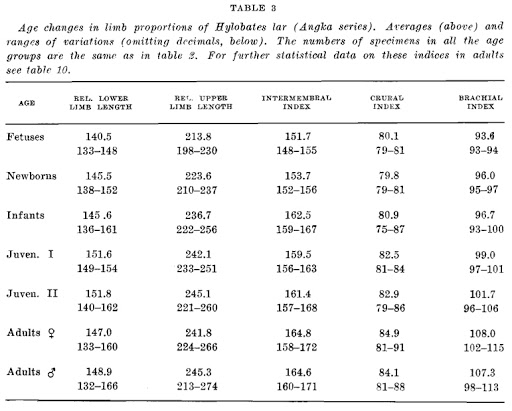
The biological significance of this pattern is difficult to discern. The length of a limb segment is determined by a number of factors, including the spacing between the initial limb condensations embryonically, and thereafter the growth rates and duration of growth at proximal and distal epiphyses. As a result, limb proportions aren’t static throughout life, but change from embryo to adult. For instance, here are limb proportion data for the coolest animal ever – gibbons! – from the great anatomist Adolph Schultz.

ResearchBlogging.orgAn important question, and follow-up to Pietak et al’s study, is whether human limb proportions can be described by such log-periodic functions throughout ontogeny, and if so how these change. Plus, it’s also not clear to what extent human proportions might happen to be describable by log periodic functions, simply because each segment is shorter than the one preceding it proximally. In short, this study raises really interesting and pursuable questions about how and why animal limbs grow to the size and proportions that they do.

References
Pietak A, Ma S, Beck CW, & Stringer MD (2013). Fundamental ratios and logarithmic periodicity in human limb bones. Journal of anatomy, 222 (5), 526-37 PMID: 23521756

Schultz, A. (1944). Age changes and variability in gibbons. A Morphological study on a population sample of a man-like ape American Journal of Physical Anthropology, 2 (1), 1-129 DOI: 10.1002/ajpa.1330020102

Pre-publication: Brain growth in Homo erectus (plus R code!)

The annual meetings of the American Association of Physical Anthropologists were going on all last week, and I gave my first talk before the Association (co-authored with Jeremy DeSilva). The talk focused on using resampling methods and the abysmal human fossil record to assess whether human-like brain size growth rates were present in our >1 mya ancestor Homo erectus. This is something I’ve actually been sitting on for a while, and wanted to wait til after the talk to post for all to see. I haven’t written this up yet for publication, but before then I’d like to briefly share the results here.

Background: Humans’ large brains are critical for giving us our unique capabilities such as language and culture. We achieve these large (both absolutely, and relative to our body size) brains by having really high brain growth rates across several years; most notable are exceptionally high, “fetal-like” rates during the first 1-2 years of life. Thus, rapid brain growth shortly after birth is a key aspect of human uniqueness – but how ancient is this strategy?

Materials: We can plot brain size at birth in humans and chimpanzees (our closest living relatives) to visualize what makes humans stand out (Figure 1).

Figure 1. Brain size (volume) at given ages. Humans=black, chimpanzees=red. Ranges of brain size at birth, and the chronological age of the Mojokerto fossil, in blue.

Human data come from Cogueugniot and Hublin (2012), and chimpanzees from Herndon et al. (1999) and Neubauer et al. (2012). The earliest fossil evidence able to address this question comes from Homo erectus. Because of the tight relationship between newborn and adult brain size (DeSilva and Lesnik 2008), we can use adult Homo erectus brain volumes (n=10, mean = 916.5 cm^3) to predict that of the species’ newborns: mean = 288.9 cm^3, sd = 17.1). An almost-recent analysis of the Mojokerto Homo erectus infant calvaria suggests a size of 663 cm^3 and an age of 0.5-1.25 years (Coqueugniot et al. 2004; this study actually suggests an oldest age of 1.5 years, but the chimpanzee sample here requires us to limit the study to no more than 1.25 years). Because we have a H. erectus fossil less than 2 years of age, and we can estimate brain size at birth, we can indirectly assess early brain growth in this species.

Methods: Resampling statistics allow inferences about brain growth rates in this extinct species, incorporating the uncertainty in both brain size at birth, and in the chronological age of the Mojokerto fossil. We thus ask of each species, what growth rates are necessary to grow one of the newborn brain sizes to any infant between 0.5-1.25 years? And from there, we compare these resampled growth rates (or rather, ‘pseudo-velocities’) between species – is H. erectus more similar to modern humans or chimpanzees? There are 294 unique newborn-infant comparisons for humans and 240 for the chimpanzee sample. We therefore compare these empirical newborn-infant pairs from extant species to 7500 resampled H. erectus pairs, randomly selecting a newborn H. erectus size based on the parameters above, and randomly selecting an age from 0.5-1.25 years for the Mojokerto specimen. This procedure is used to compare both absolute size change (the difference between an infant and a newborn size, in cm^3/year), and and proportional size change (infant/newborn size).

Results: Humans’ high early brain growth rates after birth are reflected in the ‘pseudovelocity curve’ (Figure 2). Chimps have a similar pattern of faster rates earlier on, but these are ultimately lower than humans’. Using the Mojokerto infant’s brain size (and it’s probable ages) and the likely range of H. erectus neonatal brain sizes (mean = 288, sd = 17), it is fairly clear that H. erectus achieved its infant brain size with high, human-like rates in brain volume increase.

Figure 2. Brain size growth rates (‘pseudo-velocity’) at given ages. Humans=black, chimpanzees=red, and Homo erectus,=blue.

However, if we look at proportional size change, the factor by which brain size increases from birth to a given age, we see a great deal of overlap both between age groups within a species, and between different species. Cross-sectional data create a great deal of overlap in implied proportional size change between ages within a species; it is easier to consider proportional size change between taxa, conflating ages, then  (Figure 3). Humans show a massive amount of variation in potential growth rates from birth to 0.5-1.25 years, and chimpanzees also show a great deal of variation, albeit generally lower than in the human sample. Relative growth rates in Homo erectus are intermediate between the two extant species.

Figure 3. Proportional brain size increase (infant/newborn size).

Significance: Brain size growth shortly after birth is critical for humans’ adaptative strategy: growing a large brain requires a lot of energy and parental (especially maternal) investment (Leigh 2004). Plus, in humans this rapid increase may correspond with the creation of innumerable white-matter connections between regions of the brain (Sakai et al. 2012), important for cognition or intelligence. The H. erectus fossil record (1 infant and 10 adults) provides a limited view into this developmental period. However, comparative data on extant animals (e.g. brain sizes from birth to adulthood), coupled with resampling statistics, allow inferences to be made about brain growth rates in H. erectus over 1 million years ago.

Assuming the Mojokerto H. erectus infant is accurately aged (Coqueugniot et al. 2004), and that Homo erectus followed the same neonatal-adult scaling relationship as other apes and monkeys (DeSilva and Lesnik 2008), it is likely that H. erectus had human-like rates of absolute brain size growth. Thus, the energetic and parental requirements to raise such brainy babies, seen in modern humans, may have been present in Homo erectus some 1.5 million years ago or so. This may also imply rapid white-matter proliferation (i.e. neural connections) in this species, suggesting an intellectually (i.e. socially or linguistically) stimulating infancy and childhood in this species. At the same time, relative brain size growth appears to scale with overall brain size: larger brains require proportionally higher growth rates. This is in line with studies suggesting that in many ways, the human brain is a scaled-up version of other primates’ (e.g. Herculano-Houzel 2012).

ResearchBlogging.org
This study was made possible with published data, and the free statistical programming language R.

Contact me if you want the R code used for this analysis, I’m glad to share it!

References
Coqueugniot H, Hublin JJ, Veillon F, Houët F, & Jacob T (2004). Early brain growth in Homo erectus and implications for cognitive ability. Nature, 431 (7006), 299-302 PMID: 15372030

Coqueugniot H, & Hublin JJ (2012). Age-related changes of digital endocranial volume during human ontogeny: results from an osteological reference collection. American journal of physical anthropology, 147 (2), 312-8 PMID: 22190338

DeSilva JM, & Lesnik JJ (2008). Brain size at birth throughout human evolution: a new method for estimating neonatal brain size in hominins. Journal of human evolution, 55 (6), 1064-74 PMID: 18789811

Herculano-Houzel S (2012). The remarkable, yet not extraordinary, human brain as a scaled-up primate brain and its associated cost. Proceedings of the National Academy of Sciences of the United States of America, 109 Suppl 1, 10661-8 PMID: 22723358

Herndon JG, Tigges J, Anderson DC, Klumpp SA, & McClure HM (1999). Brain weight throughout the life span of the chimpanzee. The Journal of comparative neurology, 409 (4), 567-72 PMID: 10376740

Leigh SR (2004). Brain growth, life history, and cognition in primate and human evolution. American journal of primatology, 62 (3), 139-64 PMID: 15027089

Neubauer, S., Gunz, P., Schwarz, U., Hublin, J., & Boesch, C. (2012). Brief communication: Endocranial volumes in an ontogenetic sample of chimpanzees from the taï forest national park, ivory coast American Journal of Physical Anthropology, 147 (2), 319-325 DOI: 10.1002/ajpa.21641

Sakai T, Matsui M, Mikami A, Malkova L, Hamada Y, Tomonaga M, Suzuki J, Tanaka M, Miyabe-Nishiwaki T, Makishima H, Nakatsukasa M, & Matsuzawa T (2012). Developmental patterns of chimpanzee cerebral tissues provide important clues for understanding the remarkable enlargement of the human brain. Proceedings. Biological sciences / The Royal Society, 280 (1753) PMID: 23256194

Go home, RNA, you’re drunk

(Alternate title: “circRNA censors the RNA censors?”)
When I was a kid, RNA played second fiddle to DNA. RNA was a mere intermediary between the ‘book of life’ (DNA) and the stuff the book coded for (proteins). But in the years since, RNA has shown itself to be a key player in the regulation of gene expression (shut up, DNA!). We now know of lots of kinds of non-coding RNA (ncRNA) that do lots of important things in cells, such as maintaining genomic integrity in the germ line (piRNA) and preventing messenger-RNA from being translated into protein (mi-, si- and lncRNA). Keeping track of these non-coding RNAs is tough (for me at least; I focused on fossils). Now, two in-press reports (Hansen et al., 2013; Memczak et al. 2013) show things aren’t getting any easier – apparently there’s also circular RNA (circRNA; reviewed by Kosik 2013).

Why is circRNA special? Well, for one thing, it’s two ends are joined together, forming a circle; the other types are just plain, boring, open-ended strands. Lame. Also, whereas miRNAs are involved in inhibiting gene expression (e.g., RNA interference) by binding to & helping destroy messenger RNA, circRNAs act as miRNA “sponges,” binding certain miRNA to alter their function. WHAT?!

Dammit, go home RNA; you’re drunk.

ResearchBlogging.orgSomeone smarter explaining it
Kosik, K. (2013). Molecular biology: Circles reshape the RNA world Nature DOI: 10.1038/nature11956

The papers
Hansen, T., Jensen, T., Clausen, B., Bramsen, J., Finsen, B., Damgaard, C., & Kjems, J. (2013). Natural RNA circles function as efficient microRNA sponges Nature DOI: 10.1038/nature11993

Memczak, S., Jens, M., Elefsinioti, A., Torti, F., Krueger, J., Rybak, A., Maier, L., Mackowiak, S., Gregersen, L., Munschauer, M., Loewer, A., Ziebold, U., Landthaler, M., Kocks, C., le Noble, F., & Rajewsky, N. (2013). Circular RNAs are a large class of animal RNAs with regulatory potency Nature DOI: 10.1038/nature11928

The shale revolution & lying with statistics

Is U.S. energy independence, based in part on ‘fracking’ shale deposits to access oil and gas reservoirs, just a pipe dream? A comment by JD Hughes in this week’s Nature posits just this, pointing out that production at most of these deposits declines steeply in just a few years – the industry is simply not sustainable. But why all the hype around such an unsustainable resource?

In my view, the industry practice of fitting hyperbolic curves to data on declining productivity, and inferring lifetimes of 40 years or more, is too optimistic. Existing production histories are a few years at best, and thus are insufficient to substantiate such long lifetimes for wells. Because production declines more steeply than these models typically suggest, the method often overestimates ultimate recoveries and economic performance (see go.nature.com/kiamlk). The US Geological Survey’s recovery estimates are less than half of those sometimes touted by industry.

In short, yes you can fit a line to data points (i.e. production over time; do check out the link in Hughes’ quote) to model or predict how predict how production will change over time. But this does not necessarily make these predictions valid or accurate! These ‘hyperbolic curves’ (see bottom graph from the above link) are often calculated from only five years of data, but used to predict production some 40 years down the line. And what’s more, these predicted values (i.e. points on the fitted line) are not spot-on, but have a confidence interval, a range of uncertainty in which a predicted value could be found. This interval increases drastically the further off in time you are predicting.
The point: we shouldn’t be so confident in fracking and shale reserves to help solve the U.S.’s energy problems. In fact, we should be confident (and conservative) assuming they won’t solve anything for anyone except people making money off them (and even then, only in the short term).
I’ve commented on this blog before about the importance of understanding the statistical methods one employs. In the present case, industry ‘specialists,’ whether they understood line fitting or not, erroneously used statistics to predict optimistic outcomes for US energy production. And the US government and public were eager to swallow this up hook, line and sinker.
The comment (sorry it’s behind a paywall)
Hughes, J. (2013). Energy: A reality check on the shale revolution Nature, 494 (7437), 307-308 DOI: 10.1038/494307a