My Intro to Bio Anthro course, focusing on human uniqueness, has moved from the brain to bipedalism. After the abysmally big brain, perhaps the most grotesque aspect of the human species is our wont to walk on two legs. It’s just not natural.

What a terrible biped. Image credit.
Seriously, why would an animal do such a horrid thing?

Most animals need extra help to stay upright on just two limbs. Image credit.
This peripatetic penchant is apparent in our skeletons, most visibly in our long-ass legs. And indeed, species’ limb lengths and proportions generally reflect how they tend to move around. Quadrupeds, animals that walk on four legs, tend to have roughly equally-lengthed arms and legs. Gibbons, notorious ricochetal brachiators, have insanely long arms. So for lab this week, students measured surface scans of different primates’ long bones to see if form really follows function.
Here, students try their hands at measuring long bones on surface scans of primate skeletons, and use their data to calculate indices reflecting the relative lengths of limb segments. These data will be used to test whether limb proportions can be used to distinguish different locomotor types, and to hypothesize how fossil species might have moved about.

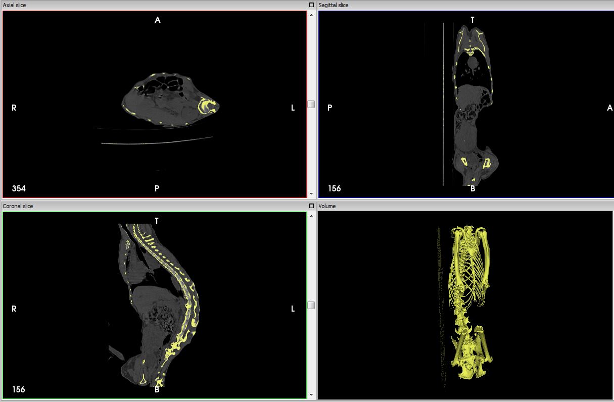
Measuring siamang (Symphalangus syndactylus) limb lengths with Meshlab. Data credit.
Since this is my students’ introduction to primate skeletons and analysis software, I only had them measure three specimens: a siamang (above), a squirrel monkey, and a grivet. But of course you can have students look at more if you wish. This activity uses the free Meshlab software and surface scans made from CT scans in the KUPRI database (surface scans are much smaller files than CT scans, making for easier dissemination to swarms of students). If you’re interested in using or modifying this activity in your class, here are the lab handout and datasheet I created for it:
Lab 2-Primate proportions
Lab 2-Primate limb data sheet
Info about, and materials for, other lab activities can be found on my Teaching page.